Index, Match, and Offset are three similar functions in Google Sheets. Also when you combine Index and Match functions, it can behave like Vlookup as well as Hlookup functions. I may bring light into that at the end of this tutorial. Before that, you should learn first the use of Index function in Google Sheets. Now here we can see how to use Google Sheets Index function.

How to Use Google Sheets Index Function

First, you should know what Index function can do or its purpose in Google Doc Spreadsheets. So here we go.

Index function can return the content of a cell based on a specified row and column offset. It’s somewhat similar to Google Sheets Offset function.

For your information, Index function has no similarity with Match function. In Match function, it returns the relative position of an item you specify. The result will be a number indicating the position.

While Index function returns an item, Match function returns relative position of an item in a range.

We can combine both these functions and use it as a flexible Vlookup. I will come to that later.

Index Function Syntax:

INDEX(reference, row, column)

Just take a look at the arguments in the Index function syntax below.

Reference: The array of cells or you can say range, to be offset into.

Row: The number of rows to offset. It’s optional and by default, it’s zero.

Column: The number of columns to offset. It’s also optional and by default, it’s also zero.

Example to Index Function:

Now let me explain you the above Index function arguments with the help of the formula in the screenshot above.

Reference: Here in this formula “A2:G12” is the array of cells or range to offset.

Row: We took 5 as the number of rows to offset. It’s marked on the image.

Column: We took 6 as the number of columns to offset. It’s also marked on the image above.

I hope the above one example is enough to learn how to use Google Sheets Index function. So let’s switch to advanced mode.

How to Use Index Function in Google Sheets Similar to Offset Function

Once you are familiar with the above example, check the below Offset function. It can return the same above result. This is just for your information.

offset(A1,5,5)

I am not going to the Offset function details here. I have already a dedicated tutorial on Google Sheets’ OFFSET function here on Info Inspired.

In Offset function, other than offset rows and columns like Index, there are Height and Width arguments. The same you can achieve using Index function also by combining two Index functions. Below are the example and comparison.

Index Vs. Offset in Google Sheets

You can skip this comparison if you are not familiar with Offset. But do try to understand the Index function used in this example.

How to Combine Match Function with Index Function in Google Sheets

When you use Match function together with Index function, it can be a killer combination. You can develop advanced look up, I mean Vlookup and Hlookup, using this combination.

See one simple example that offers dynamic vertical look up in Google Sheets. You can similarly use this combination to make horizontal look up too.

See the above screenshot. In that dataset, there is one item called “Coverall”. I know this item is there. So I can use this information to return the value of any specified cell in that row. Below is the formula.

=index(A2:G12,match(“Coverall”,C2:C12,0),7)

The above function can return the value in cell G3, that is 120, as result.

How to Combine Data in Multiple Sheets Vertically Or Horizontally by Using Index Function

I have already a data consolidation tutorial where I used query function to combine data in Google Sheets. See another way to combine data in multiple sheet tabs in google sheets using INDEX function.

Sample Data:

Combine Data Vertically Using Google Sheets INDEX function

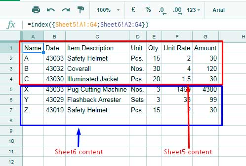
As you can see in the above image, I have two sheets with similar data set. They are “Sheet5” and “Sheet6”.

You can use the below Index formula to combine the above data. The above two sheets’ data you can combine into one sheet vertically, that means “Sheet6” data under “Sheet5”

=index({Sheet5!A1:G4;Sheet6!A2:G4})

I have used Curly Brackets here to create Array. I applied this function in a new sheet named “Sheet7”. The result will be as below.

Use the below formula when you want to combine the data horizontally.

=index({Sheet5!A2:G4,Sheet6!A2:G4})

Do remember that the range should be matching in this case.