Text, numbers, dates, times, and timestamps can all serve as criteria when using the SUMIFS function. Understanding how to utilize these diverse criteria is crucial for mastering this function.
When working with functions that involve conditions, the ability to specify criteria accurately is of utmost importance. This knowledge is key to preventing accidental errors.
I’ve noticed that many users sometimes designate a number as a string, even within IF logical tests. For instance, =IF(A1="Apple", "1", "0") is acceptable if you don’t intend to use the result in calculations. However, for calculations, it should be written as =IF(A1="Apple", 1, 0).
The SUMIFS function follows the same principle. But before delving into how to employ various criteria with SUMIFS, it’s essential to clarify the term: “Criterion.” “Criteria” is the correct plural form of the word.
What Is the Criterion in Functions
The term ‘criterion’ has its origins dating back to the 17th century, derived from the Greek word ‘kritērion,’ which means ‘judging.’ In the context of Google Sheets and functions, a criterion serves the same purpose as ‘judging.’ It represents the pattern or test applied to determine the output.
Within functions, when examining syntax elements, the term ‘criterion’ is described as ‘the pattern or test to apply.’
In simpler terms, a criterion can be likened to a condition, such as ‘if these conditions are met, then do that.’
Criteria come in various types, including text, numbers, dates, times, and timestamps. Now, let’s explore how to use these diverse criteria in the SUMIFS function.
Using Different Criteria in the SUMIFS Function in Google Sheets
We can specify different criteria in the SUMIFS function in two ways: either hardcode them within the formula or refer to a cell.
The table below will help you learn how to use different criteria in the SUMIFS function.
| Type | Hardcoding (Criterion within formula) | Value in the Cell (Criterion as cell reference) |
| Text | “North” | North |
| Number | 200 | 200 |
| Date | DATE(2023,12,31) DATE(year, month, day) | 31/12/2023 Try ‘=TODAY()’ to find the format |
| Time | TIME(17,30,0) TIME(hour, minute, second) | 17:30:00 |
| Timestamp | =DATE(2023,12,31)+TIME(17,30,0) | 31/12/2023 17:30:00 Try ‘=NOW()’ to find the format |
| Comparison | “>”&200 “>”&DATE(2023,12,31) “>”&TIME(17,30,0) | Please see examples below |
Examples
To use the formula correctly, it’s essential to understand the syntax, and here it is.
SUMIFS(sum_range, criteria_range1, criterion1, [criteria_range2, …], [criterion2, …])The purpose of this tutorial is to familiarize you with using the diverse criteria in the SUMIFS function. We will only use the first three required arguments in the function: sum_range, criteria_range1, and criterion1.
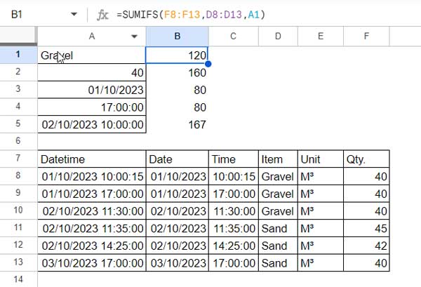
The sample data in A7:F13 has been arranged in a manner that facilitates the use of different criteria in the SUMIFS function.

We will begin by employing criteria using cell references. The different criteria are listed in the range A1:A5, and the corresponding formulas are found in B1:B5.
SUMIFS Criteria as Cell References
The formula in cell B1 uses the text criterion in cell A1. It returns the sum of ‘Qty.’ if ‘Item’ is equal to ‘Gravel.
=SUMIFS(F8:F13,D8:D13,A1)Now, let’s look at the following SUMIFS formula in cell B2:
=SUMIFS(F8:F13,F8:F13,A2)This formula sums ‘Qty.’ if it is equal to 40.
The formula in cell B3 sums ‘Qty.’ if ‘Date’ is equal to 01/10/2023.
=SUMIFS(F8:F13,B8:B13,A3)In the next formula in cell B4, we demonstrate how to use the TIME criterion in the SUMIFS function.
=SUMIFS(F8:F13,C8:C13,A4)Lastly, we introduce timestamp usage and include a comparison operator in the following formula:
=SUMIFS(F8:F13,A8:A13,">"&A5)Hardcoded
The most challenging aspect of using diverse criteria in SUMIFS in Google Sheets is using hardcoded criteria.
Here, I will hardcode the criteria in B1:B5 in the formulas below.
=SUMIFS(F8:F13,D8:D13,"Gravel")
=SUMIFS(F8:F13,F8:F13,40)
=SUMIFS(F8:F13,B8:B13,DATE(2023,10,1))
=SUMIFS(F8:F13,C8:C13,TIME(17,0,0))
=SUMIFS(F8:F13,A8:A13,">"&DATE(2023,10,2)+TIME(10,0,0))
I hope the above tips will help you master the SUMIFS function in Google Sheets.
Resources:


