


")


I am going to share with you a very rare and tricky use of AND, OR with Google Sheets Filter Function. I’m sure it will be totally new to you. What else! I am going to compare AND, OR, FILTER Formula with AND, OR, IF Logical Formula.
We have already detailed tutorials on Google Sheets FILTER, AND, OR, IF Functions. Now here I will explain to you how to use AND, OR with Google Sheets Filter Function.
So, before going to follow this very rare Google Sheets tutorial, I advise you to please go through our below spreadsheet tutorials which can make this tutorial worthy to read and easy to grasp.
Different Scenarios in AND, OR, FILTER Combination in Google Sheets
There are three different scenarios in the use of AND, OR, Filter Formula combination. What are they?
- OR – Independently with FILTER Formula.
- AND – Independently with FILTER Formula.
- AND, OR – Combined with FILTER Formula.
Let me explain to you what type of data we are going to filter using this FILTER, AND, OR combination in Google Sheets.
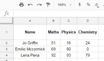
The above data shows the marks of three students out of 100 in three different subjects.
We are setting up three different conditions to find whether they are passed or failed. I mean the three scenarios in the use of Filter, AND, OR combination in Sheets.
1. The Condition or Scenario 1: Students should score more than 49 marks in any one of the subjects to pass the exam.
2. The Condition or Scenario 2: Students should score more than 49 marks in all three subjects to pass the exam.
3. The Condition or Scenario 3: Students should score more than 49 marks in any two subjects to pass the exam.
Here I am going to use FILTER, AND, OR combination to check the above three different scenarios. Also, I’m doing the same with IF, AND, OR combination.
How to Use AND, OR with Google Sheets Filter Function
OR with FILTER Function in Google Sheets (Any One Subject >=50, Passed)
Here we should use the OR logical function with Filter Formula. Once again, see the data below.
First, let us see how to deal with this using IF Logical Formula with OR.
=IF(OR(B2>49,C2>49,D2>49),"PASSED","FAILED")For the first student, we can use this formula. Then we can copy and paste this formula to down.
See how I have used OR with IF formula here. Here, if the student scored “>49” or you can say “>=50” in any subject, that student is considered as passed.
Now you can see how can we use OR with the Filter function in Google Sheets. Here is that awesome formula.
Note:
In FILTER function, you can replace the Boolean OR with Addition (+ sign). Also In FILTER function, you can replace the Boolean AND with multiplication (* sign)
Here is the use of OR with FILTER in Google Spreadsheets.
=IFERROR(FILTER(A2:D4,(B2:B4>=50)+(C2:C4>=50)+(D2:D4>=50)))Explanation with reference to Syntax:
Syntax: FILTER(RANGE, CONDITION1, [CONDITION2])Here “A2:D4” is the range and (B2:B4>=50)+(C2:C4>=50)+(D2:D4>=50) is condition # One.
Since there is no comma between OR, Google Sheets considers it as a single condition.
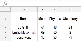
AND with FILTER Function in Google Sheets (All Subjects >=50, Passed)
Here we require to use AND with Filter Formula. Same as above, here also first let us see how this can achieve with an IF Logical Formula.
=IF(AND(B2>49,C2>49,D2>49),"PASSED","FAILED")Now see how to use FILTER with AND Logical Function in Google Sheets.
As I’ve mentioned above, you should use an asterisk sign (*) to replace the Boolean AND. So the formula will be as below.
=IFERROR(FILTER(A2:D4,(B2:B4>=50)*(C2:C4>=50)*(D2:D4>=50)))But it’s not required! A normal FILTER function can be used as below to get the same filter result.
=IFERROR(FILTER(A2:D4,B2:B4>=50,C2:C4>=50,D2:D4>=50))Both the above formula, test the range with condition whether all the marks are greater than >49.
Here lies the secret! Many advanced Google Sheets users ignore the importance of AND in FILTER as they think it’s not necessary.
The below example can tell you, how important is the AND, FILTER combination in Google Sheets.
AND, OR with FILTER Function in Google Sheets (Any Two Subjects >=50, Passed)
As earlier, first, see the combination of IF, OR, AND formula to solve the issue.
=IF(OR(AND(B2>49,C2>49),AND(B2>49,D2>49),AND(C2>49,D2>49)),"PASSED","FAILED")Now here is the advanced AND, OR, FILTER combination in Google Sheets.
=IFERROR(FILTER(A2:D4,((B2:B4>=50)*(C2:C4>=50))+((B2:B4>=50)*(D2:D4>=50))+((C2:C4>=50)*(D2:D4>=50))))Carefully check all the formulas and experiment with your own data set to learn this trick.
If you want you can copy and use my sample sheet. Below is the sample spreadsheet where I’ve used all these AND, OR with Google Sheets Filter Function variations.
If you have enjoyed this Google Sheets tutorial, please share on Facebook/Twitter and other social pages.
Additional Resources
- Regexmatch in Filter Criteria in Google Sheets (Examples).
- Comma-Separated Values as Criteria in Filter Function in Google Sheets.
- How to Use Date Criteria in Filter Function in Google Sheets.
- Use Query Function as an Alternative to Filter Function in Google Sheets.
- Filter Based on a List in Another Tab in Google Sheets.
- Two-way Filter in Google Sheets (Using Query).
Is there any way to add both types of functions for the filer?
To use criterion 1 and criterion 2 or criterion 3.
Below is what I have for two criteria that need to be inputted. But I want to make the third criterion optional or leave it blank.
=FILTER(pricebooks_data,Pricebook_name=B3,Currency=B4)The above works.
=FILTER(pricebooks_data,Pricebook_name=B3,Currency=B4 OR(Product_family=B5))It doesn’t work.
Hi, Caroline,
Here is one way to solve this.
=FILTER(pricebooks_data,Pricebook_name=B3,Currency=B4,if(B5="",row(Product_family),Product_family=B5))
Related: Select All or a Specific Category in Multiple Columns in Filter in Google Sheets.
Many thanks to you! I had similar questions / needs to Heather and Nicholas, and this was the only tutorial I found that addressed it. Much appreciated!
Hi, Milo,
Thanks for your feedback.
THANK YOU!!
I’ve been trying to find this Filter AND/OR solution for weeks in my spare time. I knew there had to be a way.
Thank you for the excellent tutorial!
I’m trying to create a filter formula with multiple OR conditions, that is more open-ended. This formula is working for me.
=filter(A3:C, (A3:A = E3)+(A3:A = E4)+(A3:A = E5))However, column E is meant to be dynamic and updating.
I have tried Query to do the same, but have run into similar issues with an open range.
The fixed range equation looks like this –
=query({Example!A3:C}, "Select * where Col1 matches "&ArrayFormula("'"&textjoin(".*|",true,".*"&E3:E5)&".*'")& "order by Col1 asc")Thank you for any help you can offer and for your excellent tutorials!
Much of what I know about Google Sheets, I have learned from your site!
Hi, Anne-Marie,
You were almost close to the solution with your Query()
Replace
E3:E5withfilter(E3:E,len(E3:E))If you want Filter(), go with this one.
=filter(A3:C, regexmatch(A3:A,"(?i)^"&textjoin("$|^",true,E3:E)&"$"))Thank you so much for the Advanced Filter AND OR combination. I tried with “,” together with “+”, but it did not work. The key was to replace the “,” with a “*” to get it to work! Thx!
Hi,
Can we use importrange with a combination of Filter and OR?
Hi, Hima,
Yes! We can do that. But not advisable because it might slow down the performance of the file (sheet).
The reason we need to use multiple importrange formulas. One importrange for ‘range’ another for ‘condition1’ and so on.
FILTER(range, condition1, [condition2, …])So better to use Query as multiple OR is easy to use in Query.