Do you know how many count functions are there in Google Sheets? Maybe not, right? There are nine count functions in Google Sheets.

Here are all nine count functions in Google Sheets:

1. COUNT
2. COUNTA
3. COUNTUNIQUE
4. COUNTUNIQUEIFS
5. COUNTBLANK
6. COUNTIF
7. COUNTIFS
8. DCOUNT
9. DCOUNTA

Now, let’s delve into how to use all Google Sheets count functions with proper examples. I’ll provide separate detailed tutorials wherever necessary.

Basic Count Functions in Google Sheets

COUNT Function

We will explore all Google Sheets count functions, starting with the COUNT function, which is the simplest among the nine count functions.

Syntax: COUNT(value1, [value2, …])

COUNT returns the number of numeric values in a range or multiple ranges. Let’s understand the COUNT function with a few examples.

Sample Data:

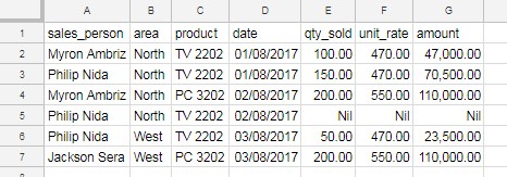
In the following sample data, we have numeric values in columns E, F, and G. However, they also contain text, which is “Nil”.

Here are a few formulas to help you easily understand the COUNT function:

1. =COUNT(G2:G7)
   This formula will return the result 5. The range in the formula covers six cells, but one cell contains a text value. The COUNT formula only counts numeric values in a given range.
2. =COUNT(E2:E7, G2:G7)
   Here, multiple ranges that are not adjoining columns are used to count. The result will be 10. This formula counts numeric values in two different column ranges.
3. =COUNT(E2:G7)
   In this formula, multiple columns are covered, but all the columns in the range are adjoining.

I hope this provides a clear understanding of how to use the COUNT function in Google Sheets.

Please note that in Google Sheets, dates are considered as numbers. Therefore, if your data includes a mix of dates and numbers, the COUNT function will count both.

How to Exclude Dates While Counting Numbers in a Column in Google Sheets

Formula:

=ArrayFormula(LET(
   range, B3:B11, 
   test, IFERROR(DATEVALUE(range)), COUNT(IF(test="", range))
))

In this formula, replace B3:B11 with the range containing the numbers you want to count, excluding text and dates.

COUNTA Function

The COUNTA function in Google Sheets is similar to the COUNT function, with the main difference being that COUNTA counts all values regardless of their data type. It only ignores blank cells.

Syntax: COUNTA(value1, [value2, …])

In the provided sample data, the formula =COUNT(G2:G7) will return 6.

COUNTUNIQUE Function

COUNTUNIQUE is an enhanced version of the COUNTA function. While COUNTA counts all values in a dataset, COUNTUNIQUE specifically tallies unique values, disregarding repetitions.

Syntax: COUNTUNIQUE(value1, [value2, ...])

Let’s assume column A contains the following values: “Apple”, “Orange”, and “Apple” in cells A1, A2, and A3 respectively.

The following formula will return 2 because the unique values are “Apple” and “Orange”:

=COUNTUNIQUE(A:A)

How to Count Distinct Values in Google Sheets

While there isn’t a specific COUNTDISTINCT function in Google Sheets, we can achieve this by combining UNIQUE and COUNTA functions.

For instance, if the values in column A are “Apple”, “Orange”, “Apple”, “Mango”, and “Banana”, the following formula will return 3, which is the count of distinct values in the range:

=LET(range, A1:A, COUNTA(UNIQUE(range, ,TRUE)))

COUNTBLANK Function

As its name suggests, the COUNTBLANK function returns the count of blank cells in the specified range. You can use this function similarly to COUNT, COUNTA, or COUNTUNIQUE.

Syntax: COUNTBLANK(range)

Example:

=COUNTBLANK(A1:A)

If column A contains 1000 rows and only three cells have values, the formula will return 997, which is the count of blank rows in column A.

Conditional Count Functions in Google Sheets

COUNTIF Function

You can use the COUNTIF function for conditional counting in Google Sheets.

Syntax: COUNTIF(range, criterion)

Examples:

1. =COUNTIF(A2:A, 110000)
   This COUNTIF formula checks a single-column range and counts the cells if the cell value is 110,000.00. The COUNTIF function allows checking only one criterion or condition at a time.
2. =COUNTIF(A1:E, ">400")
   The above COUNTIF function checks the values in cell range A1:E and counts them if they are greater than 400.

For detailed learning, please refer to this guide: COUNTIF Google Sheets Function: A to Z

COUNTIFS Function

Using COUNTIFS, you can check multiple ranges with multiple criteria. If all the conditions match, the formula will count it.

Syntax:

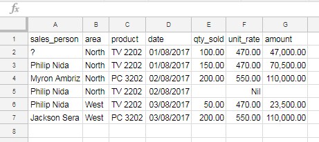
=COUNTIFS(criteria_range1, criterion1, [criteria_range2, criterion2, …])

Here is sample data in the range A1:G7 suitable for testing the COUNTIFS function.

Examples:

=COUNTIFS(C2:C7, "TV 2202", F2:F7, 470)

This COUNTIFS formula checks column range C2:C7 for “TV 2202” and matches 470 in the same row in column range F2:F7. If both criteria are met, meaning “TV 2202” is found in the same row as 470 in columns C and F respectively, they will be included in the count.

The above formula’s result will be 3 as only three rows are matching the criteria, which are rows #2, #3, and #6.

Here is one more example:

=COUNTIFS(D2:D7, ">"&DATE(2017, 8, 1), D2:D7, "<"&DATE(2017, 8, 10))

This COUNTIFS formula checks column range D2:D7 for dates between 01/08/2017 and 10/08/2017 and returns the count.

For detailed learning, please refer to this guide: COUNTIFS Array Formula in Google Sheets

COUNTUNIQUEIFS Function

The COUNTUNIQUEIFS function is relatively new in Google Sheets. Its purpose is to count unique values conditionally.

Let me explain a scenario where you will find this count function useful. Assume you are selling multiple products. The product names are in column A, and the quantities sold are in column B.

The following COUNTIF will return the count of sales where the sales quantity is greater than 10.

=COUNTIF(B1:B, ">10")

If you’re interested in knowing the count of unique products with quantities above 10, then utilize COUNTUNIQUEIFS.

=COUNTUNIQUEIFS(A:A, B1:B, ">10")

For detailed learning, please refer to this guide: How to Use the COUNTUNIQUEIFS Function in Google Sheets

DCOUNT Database Function

DCOUNT is a database function used to count numerical values, so its usage differs significantly from other count functions in Google Sheets.

It requires structured data, resembling a table, to function properly.

Syntax: DCOUNT(database, field, criteria)

• database: The table containing the data to be considered.
• field: The column to count. It can be a text label corresponding to a column header or a numeric index indicating which column to consider.
• criteria: A table containing conditions to filter the database values before operating.

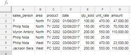
Now, let’s move on to examples. Below is the sample data (range A1:G7).

In this data, A1:G1 contains the field labels: sales_person, area, product, date, qty_sold, unit_rate, and amount, respectively.

See the formula and the criteria usage below.

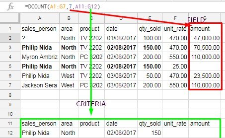
=DCOUNT(A1:G7, 7, A11:G12)

The criteria are in A11:G12 where A11:G11 contains the same field labels as mentioned above.

The DCOUNT formula above will count the occurrences in field number 7, which corresponds to the “amount” column, if the “sales_person” name is “Philip Nida”, the “area” is “North”, the date is “02/08/2017”, and the “qty_sold” is 150.

DCOUNTA Database Function

DCOUNTA is a database function similar to DCOUNT, except it counts all values irrespective of type.

Syntax: DCOUNTA(database, field, criteria)

The usage is similar to DCOUNT.

For detailed learning, please refer to this guide:: How to Use DCOUNT and DCOUNTA Functions in Google Sheets