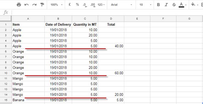
The Subtotal command in Excel enables users to add group total based on each change in a column value. At present, Google Sheets has no similar option.

In Google Sheets, the possibly best way to achieve a similar result is by using Pivot Table.

You can optionally use the QUERY function if you want the group-wise total in Google Sheets.

But all these functions and commands populate the data in a separate range in Google Sheets.

A command similar to Subtotal in Excel, as a side note SUBTOTAL function is different, is what I am missing in Google Sheets.

In a limited way, we can overcome this with a custom formula.

How to Add Total Based on Each Change in a Column Value

Sample Data:

In this Google Sheets example, there are four fruit items in column A. You can call it four groups.

To add the total based on each change in a column value, we require the items sorted, and the above sample data fulfills this criterion.

You can see the total in column D based on each change of values in column A.

To add such totals, I’ve applied a custom Google Sheets formula in cell D2 and then copy-pasted it down.

Formula:

=if(A2<>A3,sum($C$1:C2)-sum($D$1:D1),"")

Note: I have array formulas to achieve the same output. Get that here – Sum Column B When Value in Column A Changes in Google Sheets.

I know I should explain this formula so you can use it on any column in your original data.

Formula Explanation Part:

As I told you, it’s not an array formula. So, you should copy-paste it down.

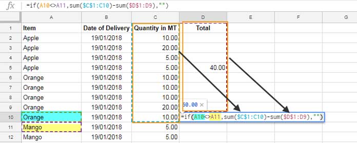
For explanation purposes, I’m taking you to the formula in cell D10. See the screenshot.

The formula in D10 tests the value in A11 whether it’s equal to the value in A10.

If the A11 value is different, in D10, the IF logical function would execute the SUM function, else return a blank.

The SUM function sums column C up to C10 and then minus any value in column D up to D9. See the above screenshot to understand it. That’s all.

The only drawback of the above formula approach to adding total based on each change in a column value is that it’s not an array formula that spills down.

Additional Info.: If you want the subtotal or grouped total, the below Query formula is enough. It populates the summary in a new range.

=query(A1:C,"select A, sum(C) where A<>'' group by A", 1)

That’s all. Thanks for the stay. Enjoy!