Here is an advanced use of Google Sheets RANK function. I’m going to provide you a custom Google Sheets formula that you can use to find Rank of a non existing number in an existing data range.
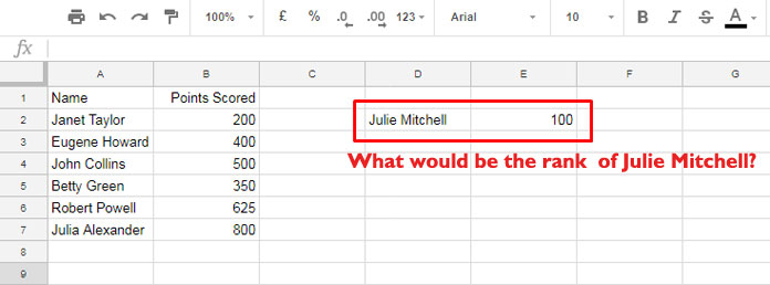
To explain this, let me directly go to an example. I’ve the score of few participants in a game as below in a Google Doc Spreadsheet.

As you know, with the help of RANK function I can easily find the RANK of each participants. I can use the following formula in Cell C2 and copy it to down.
=RANK(B2,$B$2:$B$7,0)
Now see the below image.

Now I want to find the RANK of a person named “Julie Mitchell” whose score is not yet added in the above data. Can I find the rank of this person by using the normal RANK function as below?
=RANK(100,B2:B7,0)
Nope! Normally the RANK function returns an “#N/A” error when the number is not in the selected range. To find Rank of a non existing number in an existing data range we have to use a combination of formulas.
Formula to Find Rank of a Non Existing Number in an Existing Data Range
Below is that formula.
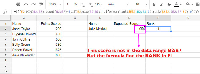
=if(E2<MIN(B2:B7),count(B2:B7)+1,if(E2>max(B2:B7),1,iferror(rank($E$2,B2:B8,0),rank($E$2,{B2:B7;E2},0))))
Note: See individual use of all the above Google Sheets Functions.
How can I use this custom RANK formula?
You can use this formula directly in your own spreadsheet. But you may want to modify the data ranges. In the above formula B2:B7 is the data range. You may want to change this range to your data range and also the value in E2 of which the rank we have to find.

Tips: To see the above formula in action, check my example spreadsheet. You can find the link at the end of this Google Sheets Tutorial.
Formula Explanation
For explanation purpose I am going to split our custom RANK formula into four parts. See the formula again below and take a note of the colour pattern.
=if(E2<MIN(B2:B7),count(B2:B7)+1,if(E2>max(B2:B7),1,iferror(rank($E$2,B2:B8,0),rank($E$2,{B2:B7;E2},0))))
1. First Part in Red Colour:
The first part of the formula in Red colour checks the value in cell E2. You can call this cell value as forecast number, would be number, or non existing number in the data range.
Here I’ve used MIN function to find the minimum value in the data range B2:B7. If the would be value in Cell E2 is less than the minimum value, that means the value in E2 is not in the data range and so it’s the lowest ranked one.
To find the lowest RANK in our data range B2:B7, I’ve used the COUNT function. The COUNT formula counts the data range and then adds 1 to it to get the last RANK.
2. Second Part in Blue Colour:
Here also, I’ve followed the same above concept. Here using the Max function, find the top RANK. If the value in E2 is greater than the values in our data range, that means E2 value is not in the range and it’s RANK is 1.
3. Third Part in Sea Green Colour:
This is a normal RANK function. If the value to check for RANK in E2 is already in the range, as usual, this part of the formula would return the actual RANK of that number.
4. The Fourth Part is in Red Violate Colour:
RANK function normally returns “#N/A” error, as said above, when the value to find the RANK is not in the range. Here in the third part of the formula, I have used IFERROR function.
If the RANK function returns error, it means the value is not in the range and also the value is between the Maximum and Minimum value in the range. So, I’ve directly added the value to existing range as below as an array by virtue of Curly Braces and then find the Rank of this range.
={B2:B7;E2}
Conclusion:
The above custom formula is not the only one that we can use to find Rank of a non existing number in an existing data range. You can achieve the above same result with a Vlookup and RANK combo formula as below.
=RANK(E2,IF(ISERROR(vlookup(E2,B2:B7,1,FALSE))=TRUE,{B2:B7;E2},{B2:B7}))
I don’t know how many of you use such type of formulas in real life situations. If you use, I wish to hear form you in comments about the purpose of use.
Update
You can directly use the below formula. There is no logical test require.
=RANK($E$2,{B2:B7;E2},0)


