


")


In Google Sheets, extracting a date from a timestamp can be done using various functions. Here, we present the 5 easiest methods.
Learning this technique is crucial, especially when you need to lookup a date in a timestamp column or use FILTER or QUERY to filter a timestamp column based on date criteria.
You can utilize one of the formulas below for this purpose, converting timestamps to dates and enabling their use in lookups or filters.
How to Extract a Date From a Timestamp in Google Sheets
For the examples, let’s consider the datetime (timestamp) in cell A1, which is “05/08/2023 13:50:29”. The formulas provided will work seamlessly, even if the timestamp contains milliseconds, such as “05/08/2023 13:50:29.231”.
You May Like: How to Remove Milliseconds from Timestamps in Google Sheets
Please note that the result of the formulas will be a date value. You need to format it as a date by navigating to the cell containing the formula (date value) and clicking “Format > Number > Date.” Alternatively, you can wrap the formula with the TO_DATE function.
Now, let’s explore the five formulas to extract a date from a timestamp:
Formula 1 Using INT Function:
=INT(A1)The INT function rounds down a value to the nearest integer, which applies to a timestamp. In a timestamp, the time component is treated as the fractional part.
Formula 2 Using TRUNC Function:
=TRUNC(A1)The TRUNC function uses ‘value’ and ‘places’ arguments. If ‘places’ are omitted, it truncates all decimal places, making it suitable for extracting dates from timestamps in Google Sheets.
Formula 3 Using the ROUNDDOWN Function:
=ROUNDDOWN(A1)Rounding down a number to 0 places returns the whole number. This can be used effectively to extract a date from a timestamp.
Formula 4 Using FLOOR Function:
=FLOOR(A1)The FLOOR function rounds a number down to a specified multiple. It requires two arguments: ‘value’ and ‘factor.’ If you omit the ‘factor,’ it defaults to 1. Therefore, the above formula is used to extract the date from the timestamp in cell A1.
Formula 5 Using the DATEVALUE Function:
=DATEVALUE(A1)This DATEVALUE formula has certain advantages over the previous ones. The datetime in cell A1 must be a recognized date format and can also be a date string. It ensures the return of the date component only. Unlike other formulas, if cell A1 contains a number instead of a timestamp, it will return an error.
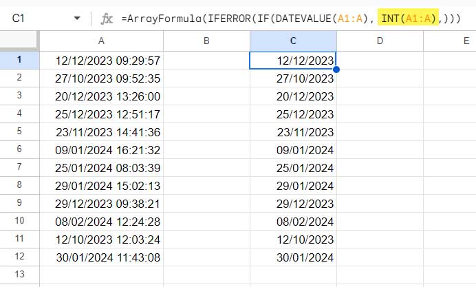
Next, we will convert these formulas into array formulas to transform timestamps in a column into dates.
Transforming Timestamps in a Column into Dates
To transform timestamps in a column into dates, you can follow this generic formula for Formulas 1 to 4:
=ArrayFormula(IFERROR(IF(DATEVALUE(A1:A), your_formula,)))Replace your_formula with the formula you prefer. For example, if you want to use the TRUNC function, replace your_formula with TRUNC(A1:A).
Example:
=ArrayFormula(IFERROR(IF(DATEVALUE(A1:A), TRUNC(A1:A),)))The IF(DATEVALUE(A1:A) part tests if the provided range contains valid dates, then truncates the decimal parts; otherwise, it returns errors. The IFERROR is used to remove those errors.
However, for the fifth formula, you can simply use the following formula:
=ArrayFormula(IFERROR(DATEVALUE(A1:A)))Formulas to Extract Time from a Timestamp
We’ve already covered how to extract dates from timestamps in Google Sheets. Now, let’s explore how to extract time from a timestamp.
You can use either the MOD function or the SPLIT and CHOOSECOLS combo to achieve this in Google Sheets.
To extract the time from the datetime in cell A1, you can use the following formula:
=MOD(A1, 1)The MOD function returns the remainder after a division operation. In this case, the divisor is 1, and the dividend is the datetime in cell A1. The result will be the fractional part, which represents the time component.
Make sure to format the result as time using “Format > Number > Time.”
Another option involves the SPLIT operation, which separates the datetime into date and time. The CHOOSECOLS function allows you to choose either the date or time, as desired.
=CHOOSECOLS(SPLIT(A1, " "), 1) // will return the date
=CHOOSECOLS(SPLIT(A1, " "), 2) // will return the time
We can convert both of these formulas (MOD and SPLIT-CHOOSECOLS combo) into array formulas:
=ArrayFormula(IFERROR(IF(DATEVALUE(A1:A), MOD(A1:A, 1),)))
=ArrayFormula(CHOOSECOLS(SPLIT(A1:A, " "), 2))
Resources
We have 5 formulas to extract dates from timestamps and two formulas to extract time from timestamps in Google Sheets. Additionally, we have explored the array formula versions of these functions.
Here are some timestamp-related resources.
- How to Compare Time Stamp with Normal Date in Google Sheets
- How to Filter Timestamp in Query in Google Sheets
- Google Sheets: The Best Overtime Calculation Formula
- COUNTIFS in a Time Range in Google Sheets
- How to Convert Military Time in Google Sheets
- How to Use DateTime in Query in Google Sheets
- Elapsed Days and Time Between Two Dates in Google Sheets
- How to Increment Time By Minutes and Hours in Google Sheets
- How to Convert Timestamp to Milliseconds in Google Sheets
Greetings,
Having some issues where trying to extract a date from a timestamp generated by merchant service device returns an incomplete date with formula.
Example:
Payment date | Extracted Date
30-Apr-2023 02:01 PM PDT | 30-Apr-202
Tried these 2 functions, and they both return the year cut-off like the example above when trying to extract.
1)
=MID(A1,FIND("-",A1,1)-2,10)2)
=MID(A1,SEARCH("??-???-",A1),10)Not sure what I’m doing wrong, but any help is greatly appreciated!
Hi, grangthony,
You can try this SPLIT + CHOOSECOLS combo.
=choosecols(split(A1," "),1)Another option is REGEXEXTRACT, but the result will be text formatted.
=REGEXEXTRACT(A1,"(\S+)")Hi Prashanth,
I am using the IFS function for automatic date filling in Google Sheets.
=IFS(AB1="","",AC1="",NOW(),TRUE,AC1)But the formula is showing yesterday’s date, not today’s date.
Hi, Manikandan Selvaraj,
It doesn’t make sense to me. Can you please explain the type of values in the relevant cells, i.e., in AB1 and AC1?
Whether they are dates, numbers, or texts?
Hi Prashanth,
Sure, AB1 contains drop-down TEXTS.
When the user changes the status text on the AB column, the AC column automatically captures the current date.
But here the issue is it captures yesterday’s date, not the current date. For reference:
AB | AC
User Status | Status Date
Completed | 25/06/2022
Ongoing | 26/07/2022
Hi, Manikandan Selvaraj,
Please see if this help?
=if(AB1="Completed",today()-1,today())I want to use a Vlookup for the date only in a timestamp, can I embed something in the formula that only reads the date or do I need a helper column that uses
=TO_DATE(INT(A1))?Hi, Phil,
I’ll post an example soon and notify you here!
Hi, Phil,
Here is the post link – Vlookup Date in Timestamp Column.
Thank you so much 🙂
Is there a way to get the result in two columns? In one column date and in another column text.
12-Jan-20 Brazil
5/6/2020 Canada
Like above?
I just want to split the dates in one column and strings in the next column.
Maybe this one?
=ArrayFormula(TO_DATE(IFERROR(split(A1:A," "))))If not working, you can share a demo sheet as earlier.
Hi,
How do I get only dates from the list of a column?
Example: in ColumnA I have;
Aus
CAN
1/2/2019
UNI
5/6/2020
In the next column, I should get only 1/2/2019 & 5/6/2020. Is there any way to extract only dates? Please help me.
Hi, Hima,
Try the below Filter + Datevalue combo.
=Filter(A1:A,datevalue(A1:A))The function DATEVALUE normally requires ARRAYFORMULA in a range (List). But when using within Filter, it’s not required.
Thank you so much. I was sick because of this problem. All the time I was adding another column next to the date and using
=Leftand=rightfunctions. Your 3rd formula worked perfectly with=ARRAYFORMULA(TO_DATE(DATEVALUE((List1!A3:A)))Thank you.
Hi, Ahmet,
Thanks for your feedback!