Maybe you have sufficient reasons to compare two sheets in Google Sheets for the mismatch. Whatever it may be, you can easily do it. In Google Sheets, there is no built-in option for comparing two similar sheets for the mismatch.

No matter how many columns are there in the sheets to find differences, you can do it hassle free with a formula.

In Google Sheets, it’s pretty easy to compare two tables side by side when it’s on the same sheet. First, we will see how to compare two tables side by side on the same sheet. Then we can move to compare two sheets to find Mismatch.

First, let us see how to compare two tables in the same sheet for the mismatch.

Find Mismatch in Two Columns Side by Side

You can use any of the below formulas when you want to find differences in two similar columns side by side. The first formula uses the IF logical function while the second one the SWITCH logical function.

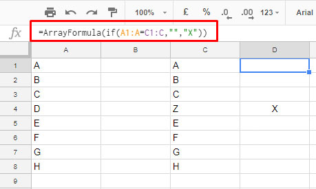
=ArrayFormula(if(A1:A=C1:C,"","X"))

OR

=ArrayFormula(SWITCH(A1:A,C1:C," ","X"))

Here I’m comparing two columns, columns ‘A’ and column ‘C’ side by side. Here data start from Row 1. So the formula should be entered in Row 1, but any columns other than Column A and C.

Here, by virtue of the ArrayFormula, you only need to key in the formula in one cell. It will automatically get expanded below. Wherever mismatches occur, it would leave an ‘X’ mark in the corresponding row.

You May Also Like: Match Two Columns that Contain Values Not in Any Order Using Regex

How to Compare Two Tables Side by Side in Google Sheets to Find Mismatch

When you want to compare a table with more than two columns side by side in Google Sheets, here is the formula.

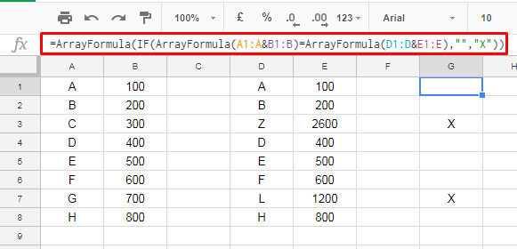
=ArrayFormula(IF(ArrayFormula(A1:A&B1:B)=ArrayFormula(D1:D&E1:E),"","X"))

The above formula compares two tables with two columns each.

How to use this comparison formula for your purposes?

In this formula, you may want to make changes in two places.

Table 1 data range.

A1:A&B1:B

Table 2 data range.

D1:D&E1:E

When you want to compare three or more column data set, the above range would be likeA1:A&B1:B&C1:C for the first table andD1:D&E1:E&F1:F for the second.

Note: I have two data ranges. One in Sheet1 and the other in Sheet2. Some of the rows in the Sheet1 range have the match in Sheet2 range.

I want to extract the mismatching rows in Sheet1. In this case, I have a different tutorial – Compare Two Sets of Multi-Column Data for Differences in Google Sheets.

The Steps to Compare Two Sheets in Google Sheets for Mismatch

Here we are going to compare the entire two sheets for differences. So definitely a third sheet is required to point out the differences or mismatch unless you go for conditional formatting.

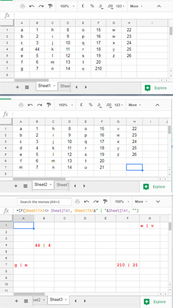
=IF(Sheet1!A1<> Sheet2!A1, Sheet1!A1&" | "&Sheet2!A1, "")

The above is that magical formula to compare two sheets for a mismatch in Google Sheets.

You should add this formula in the very first cell of your third sheet. Then copy and paste the formula to each and every cell in that sheet. You can limit the copy paste as per your data ranges in Sheet 1 or Sheet 2.

How the sheet comparison for mismatch taken place. See the screenshot which is in Sheet 1, Sheet 2 and Sheet 3 order.

The formula in sheet three found four mismatches between Sheet 1 and Sheet 2. It points out the same in corresponding cells with values from sheet 1 and sheet 2. The values in Sheet 1 and Sheet 2 are separated by “|” the pipe symbol.

Conclusion

You have learned the following data table comparison in Google Sheets.

1. Compare two columns in the same sheet for the difference.

2. Compare more than two columns in the same sheet to find the difference.

3. Compare two sheets in Google Sheets for a mismatch.

That’s all for now. Enjoy!