


This comprehensive guide walks you through the process of seamlessly adapting non-regional Google Sheets formulas to your locale, ensuring error-free operation.
For instance, in VLOOKUP, I typically follow the syntax VLOOKUP(search_key, range, index, [is_sorted]), where a comma serves as the delimiter, or we can call it the argument separator.
However, some of you may be using the same function with a different syntax, such as VLOOKUP(search_key; range; index; [is_sorted]), where the semicolon acts as the argument separator.
The usage of these formula delimiters depends on your Sheets’ locale, accessible in the File menu > Settings.
If you’re from a region different than mine, like any EU country such as France, Germany, Spain, etc., copying a formula from my tutorials might result in a formula parse error on your sheet because I have set the UK as the locale.
To resolve this issue, you can follow one of two steps:
- Change your Sheet’s locale to the UK, insert my formula, and then revert the locale back to yours.
- Adjust the formula by changing the comma separator (formula delimiter) to a semicolon.
This post guides you on how to modify a non-regional Google Sheets formula to match your locale, offering insights into adapting Google Sheets formulas for locale-specific formatting.
How Google Sheets Language and Locale Settings Impact Formulas
Two crucial settings influence formulas in Google Sheets: ‘Language’ and ‘Locale.’
The former pertains to language, while the latter is associated with date, currency, and number formatting.
The challenge arises within the ‘Locale’ settings. In certain countries, a comma serves as the standard decimal separator (e.g., €6,00) instead of a period. Consequently, using a comma as the argument separator in formulas can lead to issues; therefore, you must use the semicolon as the argument separator.
Upon accessing shared Google Sheets from a different locale, you may notice changes in the formula, such as the use of a comma instead of a semicolon or vice versa.
If sharing settings permit, making a copy of the sheet allows you to use it without complications since the sheet’s locale remains unchanged.
This ensures that existing formulas continue to function smoothly. However, when you copy-paste a formula from a sheet set to a different locale, it might not work if Google Sheets fails to correct it automatically.
Adapting a Non-Regional Google Sheets Formula to Your Locale
In the first example, the locale is set to the UK, where a comma serves as the argument separator.
Here are examples of using two popular functions: COUNTIF and VLOOKUP.
=COUNTIF(A2:A, "Apple")
=VLOOKUP("C", E2:F5, 2, 0)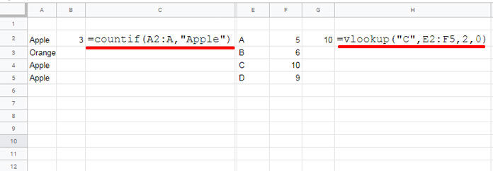
In another sheet, the locale is set to Spain.
Here are the same COUNTIF and VLOOKUP formulas with the function argument separators modified from comma to semicolon.
=COUNTIF(A2:A; "Apple")
=VLOOKUP("C"; E2:F5; 2; 0)
Observe how the formula separator changes in each locale.
Locale Settings and the QUERY Function
When using the QUERY function, errors may occur when transitioning a non-regional Google Sheets formula to your locale.
To illustrate, examine the QUERY syntax in two different locales:
QUERY(data, query, [headers])
QUERY(data; query; [headers])
The argument separators are, of course, the comma or semicolon. However, the column ID separators must be a comma, not a semicolon. When using native functions within the query string, they should follow the comma/semicolon settings.
Let’s consider two examples:
=QUERY(A1:D, "select A, sum(C), B where A is not null group by A, B", 1)
=QUERY(A1:D; "select A, sum(C), B where A is not null group by A, B"; 1)
In these two QUERY formulas, the first one has the locale set to UK, and the second one has the locale set to Spain. The argument separators are a comma or semicolon, depending on the locale, but within the query string, the column identifiers are separated by a comma in both.
Now, observe two more formulas:
=QUERY(A1:D, "select A, B where D=date '"&TEXT(D2, "yyyy-mm-dd")&"' ", 1)
=QUERY(A1:D; "select A, B where D=date '"&TEXT(D2; "yyyy-mm-dd")&"' "; 1)
The difference lies in the worksheet function used within the query string. They should follow the locale setting.
How Locale Settings Impact Separators in Array Creation
You can effortlessly create arrays in Google Sheets by enclosing a set of values within curly braces.
In UK locale settings, use a comma separator to create an array by row (HSTACK) and a semicolon to create an array by column (VSTACK).
Example for Array By Row:
={B2:C4, E2:F4}Example for Array By Column:
={B2:C4; E2:F4}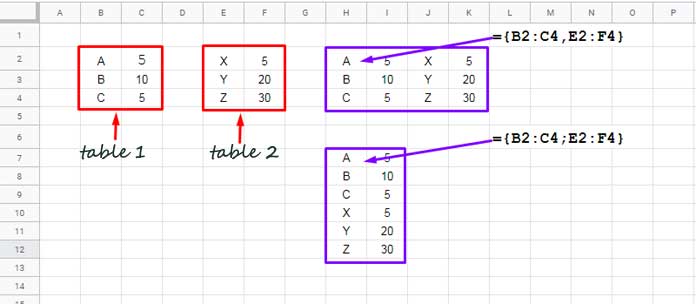
In the case of Spain, the comma should be replaced by a backslash. No changes to the semicolon.
Example for Array By Row:
={B2:C4\ E2:F4}Example for Array By Column:
={B2:C4; E2:F4}Conclusion
In summary, here are the key takeaways from this tutorial:
- When converting a non-regional Google Sheets formula to your locale:
- Replace argument separators from a comma to a semicolon or vice versa.
- In the QUERY function, the separators (column identifier separators) within the query string must be a comma.
- In the QUERY function, any formula used within the query string must follow point #1 above.
- When creating arrays, a comma must be replaced by a backslash or vice versa.