How to Highlight Cells Based on Expiry Date in Google Sheets

In a spreadsheet, a highlighted cell can draw your attention to the content within, alerting you to an important date, milestone, or something similar. Before explaining how to highlight cells based on the expiry date in Google Sheets, let me provide some context.

I maintain a Google Sheets file to record my income, daily expenses, and other crucial information such as the due date of my insurance premium, domain and hosting plan expiry dates, etc. Each category has its sheet tab.

I use conditional formatting in some sheet tabs to easily check the expiry dates of my domain registration, insurance premium, etc., as these dates are vital for me.

In sheet tabs containing such data, I’ve applied conditional formatting rules to highlight cells with two different colors based on the expiry duration.

I set the cell color to Green if the expiry dates are after one month. However, if the expiry dates are within one month, I set the highlighting to Red.

This system proves beneficial, saving me the effort of checking all dates individually. At a glance, I can determine whether I’m within a safe timeframe for my registrations and due dates.

Now, let’s delve into how to highlight cells based on the expiry date in Google Sheets. You’ll learn a simple yet effective conditional formatting rule that utilizes the Google Sheets EDATE function.

How Can This Expiry Date-Based Conditional Formatting Be Useful to You?

You can apply the expiry date-related conditional formatting in Google Sheets in various cases. Here are a few examples:

Visually identifying the expiry dates of your company registration certificates or documents.
Tracking your or your employees’ passport and driving license expiry.
Highlighting the due dates of your kids’ school fees.
Managing credit card due dates.
Keeping track of your insurance premium due date.
Ensuring timely loan repayments.
For bloggers managing multiple blogs, it helps to easily track upcoming hosting and domain expirations.

There are countless situations where you can use expiry duration-related conditional formatting in Google Sheets.

Timely payment of fees or service charges can not only save you money by avoiding late fees but also enhance your trustworthiness.

Tips to Highlight Cells Based on Expiry Date in Google Sheets

As mentioned at the beginning, the Google Sheets EDATE function can be employed here. While I’ve already provided a detailed tutorial on all Google Sheets date-related functions, I’ll go through the EDATE function once more here.

Make sure to check: Learn all Google Sheets Complete Date Functions in One Place.

I will guide you through the usage of EDATE in Google Sheets with simple examples, eliminating the need for you to refer back to my previous tutorial.

Syntax and Arguments:

EDATE(start_date, [months])

Returns a date that is a specified number of months (months) before or after a specified date (start_date).

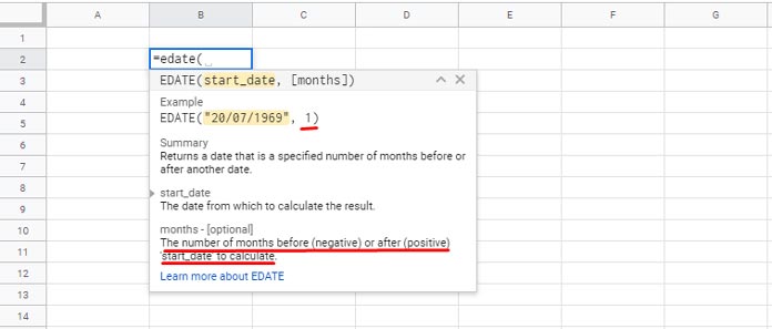
Examples:

Cell A1 contains the date 31/12/2017. Check the EDATE function below and its output.

=EDATE(A1, 1) // returns 31/01/2018

Another formula:

=EDATE(A1, 2) // returns 28/02/2018

Similarly, this function can also return the date before the referenced date.

=EDATE(A1, -1) // returns 30/11/2017

Now, let’s return to our tutorial and explore how I am going to use the EDATE function to highlight cells based on the expiry date in Google Sheets.

Method One: Expiry Date-Based Conditional Formatting Using Formula in Preset Rules

I am applying this conditional formatting to column A in the range A1:A5. You can apply it to the range you prefer.

If you’re looking for the formulas and how to use them, here they are:

Formula:

=EDATE(TODAY(), 1)

Please refer to the screenshot below, where I’ve set three custom rules (formulas) in the Format menu > Conditional formatting. All use the same formula, but the application is different.

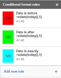
Expiry Date-Based Conditional Formatting Rules: Presets

a. Expiry Date Within One Month (Red Color):

Within the “Conditional format rules” panel, under “Apply to range,” enter A1:A5.
Select “Date is before,” then “Exact date” under “Format rules.”
Enter the EDATE formula.
Under “Formatting style,” select Red Fill color and click “Done.”

b. Expiry Date After One Month (Green Color):

Under “Apply to range,” enter A1:A5 (you might want to click “Add another rule first”).
Select “Date is after,” then “Exact date” under “Format rules.”
Enter the EDATE formula.
Under “Formatting style,” select Green Fill color and click “Done.”

c. Expiry Date in Exactly One Month (Cyan Color):

Under “Apply to range,” enter A1:A5 (you might want to click “Add another rule first”).
Select “Date is,” then “Exact date” under “Format rules.”
Enter the EDATE formula.
Under “Formatting style,” select Cyan Fill color and click “Done.”

If any of the cells are highlighted with the Red Color, it means the due date is within one month, indicating that you should take care of that payment. If it’s Green, you can simply ignore such cells.

The Explanation for the Rules Applied:

If today’s date is 19/01/2024:

Wherever the dates are less than 19/02/2024 (indicating within one month), the formula (formatting rule) would highlight those cells in column A (A1:A5) with a Red color.

If any of the dates in column A is 19/02/2024, that cell would be highlighted with a Cyan color.

If any of the dates in column A are greater than 19/02/2024, the formula would highlight those cells in column A with a Green color.

This way, you can highlight cells based on the expiry date in Google Sheets.

The above conditional formatting is based on a one-month cut-off date. If you want to set a 6-month cut-off date, just change the custom formula as below:

=EDATE(TODAY(), 6)

So the highlighting would be expiry within 6 months, on exactly the 6th month, and expiry after 6 months.

Method 2: Expiry Date-Based Conditional Formatting Using Custom Formula

The above conditional formatting rules have certain limitations, most importantly, they can test the dates only within the “Apply to range.” For example, you can’t use them to match a date in one cell for expiry and highlight another cell.

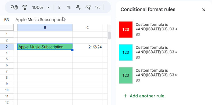
Example:

I have the subscription date of Apple Music in cell C3. I want to highlight cell B3, which contains the description of the subscription, namely “Apple Music Subscription.” How do we do that?

First, take a look at the formulas below:

=AND(ISDATE(C3), C3 < EDATE(TODAY(), 1)) // expiry within one month
=AND(ISDATE(C3), C3 > EDATE(TODAY(), 1)) // expiry after one month
=AND(ISDATE(C3), C3 = EDATE(TODAY(), 1)) // expiry exactly in one month

The formulas match if the value in cell C3 is a valid date, and also the date is within one month, after one month, or exactly one month of expiry.

You need to apply the formulas one by one as before, but within “Custom formula is” under the “Format rules” in Conditional formatting.

The “Apply to range” can be B3 if you only have one date in cell C3.

Expiry Date-Based Conditional Formatting Rules: Custom Formula Rules

If you have more subscription dates in C3:C, the “Apply to range” must be B3:B. No changes in formulas.

Also, and most importantly, if you want to highlight entire rows in the “Apply to range,” for example, B3:Z3 instead of just B3, replace all occurrences of C3 in the formulas with $C3.

Resources

This tutorial explores two approaches to highlight cells based on expiry dates in Google Sheets. Here are additional tips on Conditional formatting that will help you add more rules.

Keep in mind that applying Conditional formatting to a larger range can slow down the processing of your sheets.

102 COMMENTS

Heath June 24, 2022 At 4:12 am

I need some help. I have tried the formulas in other comments, but they are not working.

Need one cell to change multiple colors depending on date range Month/Year.

White if the date is under 11 months.
Yellow if it’s one month from being due.
Orange if it’s 1 yr due.
Red if over 1 yr and stays red until the date it updated

- Prashanth June 24, 2022 At 10:57 am
  
  Please share a spreadsheet URL in your reply. So I can insert the rules.
  
Ayumi February 17, 2022 At 6:12 pm

Hi Prashanth,

I hope you’re doing great!

I have dates from F20 cell to F100, and I want them to change colors with the following conditions.

1. Turn red if it’s already four months due from the date in F20.

2. Turn Yellow 7 days before the 4th month due date.

I hope you can help!

Thank you!

- Prashanth February 18, 2022 At 10:31 am
  
  Hi, Ayumi,
  
  I assume you want to highlight dates in F21:F100 based on the date in F20 as per the given two conditions.
  
  Rule 1 (Red)
  
  =gte(F21,edate(F$20,4))
  
  Rule 2 (Yellow)
  
  =gte(F21,edate(F$20,4)-7)
  
  - Ayumi February 18, 2022 At 4:24 pm
    
    Hi Prashanth,
    
    Sorry for the misunderstanding.
    
    E.g.:-
    
    The date in column F is Feb 18, 2022.
    
    So it will turn red when it’s May 18, 2022, and will turn yellow if it’s already May 11, 2022.
    
    - Prashanth February 20, 2022 At 3:25 pm
      
      Hi, Ayumi,
      
      Thanks for the clarification. Here are the rules for the column range F2:F.
      
      Rule # 1 (Red)
      =and(len(F2),gte(days(today(),F2),120))
      Rule # 2 (Yellow)
      =and(len(F2),gte(days(today(),F2),113))
      
      Add rule # 1 first, then rule # 2. Otherwise, the Yellow will overwrite Red.
      
      - Dilju Sunil June 7, 2022 At 4:30 pm
        
        Hi Prasanth,
        
        Can you help me with this?
        
        I want to highlight the data which repeats within 30 days. A column contains the date, and the B column contains objects.
        
        I want to highlight the objects in the B column if it appears again within 30 days.
        
        If the repetition is more than 30 days, then another color or white.
      - Prashanth June 8, 2022 At 11:22 am
        
        Hi, Dilju Sunil,
        
        We may be able to solve that using the below formula.
        
        =and(len(B2), ArrayFormula(countifs($B$2:B2&eomonth($A$2:A2,0), B2&eomonth(A2,0),lte(row($B$2:B2),row(B2)),true))>1)
        
        Try it. If that doesn’t solve, share a sample sheet (URL) via reply below.
        
        (Highlights not within one month, but in the same month)
Lindi February 9, 2022 At 6:47 pm

Hi there,

I have read all the comments and tried all the formulas, but I am not getting it to work.

I have certificates on a sheet stating the expiry dates. I need the cells to turn red 40 days before expiry.

I hope you can assist.

- Prashanth February 10, 2022 At 10:47 am
  
  Hi, Lindi,
  
  This formula is for the range C2:C.
  
  =and(len($C2),lte($C2,today()+40))
  
  Feel free to modify LTE (less than or equal) to LT (less than).
  
Reghie November 16, 2021 At 4:08 pm

Hello, can you please help me?

My client wants to make the date red if it’s 15 days passed.

For example, he inputted November 2, 2021, which is still in the original format. So when it’s November 17, 2021, it will become red and bold.

Do you know how to do this?

- Prashanth November 17, 2021 At 10:08 am
  
  Hi, Reghie,
  
  =gte(today(),B2+15)
  
  Assume cell B2 contains the date November 2, 2021.
  
Peter J Powell October 26, 2021 At 1:25 am

Maybe I didn’t see the answer in this thread, but here is what I am trying to accomplish!

I want to set up three color codes.

1) that is within a year of the certification date. I.e., if the certification happened on 25-Oct-21, then it expires on 25-Oct-22. I want it to stay green for 11 months.

2) The last month of the certification I want to turn yellow, thus letting me know it will expire in one month

3) When the certification has expired.

Everything I have tried has failed. Every client will have a different certification date.

Please Help.

- Prashanth October 27, 2021 At 9:32 am
  
  Hi, Peter J Powell,
  
  Assume the certification dates are in the cell range D2:D10. Then please follow the below steps.
  
  Select D2:D10 > Format > Conditional Formatting > Format Rule > Custom Formula Is.
  
  1. Green
  
  =LT(today(),edate(D2,11))
  
  2. Red
  
  =and(isdate(D2),GT(today(),edate(D2,12)))
  
  3. Yellow
  
  =isdate(D2)
  
  Add the rules in the above order one by one.
  
Katherine Clarke July 31, 2021 At 9:58 am

Hi Prashanth, this is a great website with tons of information, but I still can’t find what I’m looking for.

I’d like to conditionally format a cell if today’s date is past a certain date.

I am a piano teacher trying to keep track of my monthly payments. Right now, I have it formatted with each student’s name in a row and each month in a column with checkboxes.

So for my July column, if a student hasn’t paid by 2 August 2021, I’d like the cell to turn red until I click the checkbox. Do you know if I can do this?

Thanks in advance!

P.S. Not super comfortable sending my spreadsheet link as it has a few pages of student’s personal information. If necessary, I can create another blank spreadsheet to test formulas on.

- Prashanth July 31, 2021 At 11:05 am
  
  Hi, Katherine Clarke,
  
  It seems possible.
  
  Since the formula depends on many factors such as your data layout/formatting, Sheet’s Locale, etc., I won’t be able to suggest one.
  
  So, feel free to share a sample sheet below.
  
  - Katherine Clarke August 8, 2021 At 4:37 am
    
    Hi Prashanth! Thanks for your help.
    I added a row for the due date because payment is due the following month on the 1st.
    How can we adjust it? So that it is due the following month, not the first day of the stated month of payment? Thanks!
    
    - Prashanth August 9, 2021 At 10:23 am
      
      Hi, Katherine Clarke,
      I have modified the formula as below.
      =and(month(today())=month(edate(B$1,1)), year(today())=year(edate(B$1,1)),B2=FALSE)
      Read it as;
      If the month of today is equal to the month of B1+1 month (same with the year) and B2 is FALSE.
      
Stoyan June 21, 2021 At 5:07 pm

Hi all,

First of all, thank you for the rich information here.

I couldn’t find a case in the comments that are similar to mine. So I am forced to leave a comment, in the hope that you can help me also.

I have a sheet, and in column K from row 5 downwards, I enter dates on which the last reminder was sent to a stakeholder in my company. I want to highlight that cell red if more than 14 days have passed from the date entered in the cell.

For some reason, I can’t make it work. Can you help me?

Thanks

- Prashanth June 22, 2021 At 10:31 am
  
  Hi, Stoyan,
  
  Here is the formula for the range K5:K.
  
  =and(days(today(),K5) > 14,len(K5))
  
  If it doesn’t work, please try =and(days(today();K5) > 14;len(K5))
  
  - Stoyan June 22, 2021 At 1:28 pm
    
    Thank you, Prashanth! Works very good – you’re the best 🙂
    
Paige Brown June 2, 2021 At 6:45 am

Hi Prashanth,

First, thank you for all of the help you share with everyone!

I was recently hired for a position in the medical field which uses sheets regularly.
Background:

Each patient is in a different phase of treatment.
We submit authorization requests to the funding source and insert the submission date into one column ( Column A).
The adjacent column (Column B) remains blank until we receive our treatment authorization.

Goal: We’d like the cells in Column B to be highlighted if there is not yet a “Received” date in Column B:

* RED if the “Submission” date in Column A has been exceeded by 14+ days.
* ORANGE if the “Submission” date in Column A has been exceeded by 7-13 days.
* CLEAR/WHITE/OFF if we have received authorization and have input a “Received” date into Column B.

Thank you, in advance, for any assistance you are able to share; it will be appreciated for a VERY long time to come!

- Prashanth June 3, 2021 At 11:22 am
  
  Hi, Paige Brown,
  
  Try the following formulas in the Custom Formula field.
  
  RED:
  =and(len(A2),not(isdate(B2)),DATEDIF(A2,Today(),"D")>13)
  
  ORANGE:
  =and(len(A2),not(isdate(B2)),DATEDIF(A2,Today(),"D")>6,DATEDIF(A2,Today(),"D")<14)
  
  CLEAR/WHITE/OFF:
  No need to use any rules.
  
  Important!
  
  The "Apply to range" must be B2:B, not B1:B.
  
Nic Boz May 19, 2021 At 10:22 pm

I am trying so hard to make this work and it just isn’t clicking. I have a column of court hearing dates. The top row is frozen. I want each time a date is within a month for the text to turn orange. I feel like I have tried every example in the article and in the comments. The only results being either nothing changes or all my dates turn orange. Please help!

- Prashanth May 20, 2021 At 9:56 am
  
  Hi, Nic Boz,
  
  If possible, share the URL of your sheet, I will try to help.
  
  You can use the “Reply” below to share the URL which won’t be published.
  
  - Nic Boz May 22, 2021 At 2:32 am
    
    Hey Prashanth, Here is the link to help the code that makes all my hearing dates turn orange as soon as they are within a month.
    
    — link removed —
    
    - Prashanth May 22, 2021 At 2:28 pm
      
      Hi, Nic Boz,
      
      The dates to highlight are in F2:F. So the below rule for this “apply to range” will highlight any dates in this range that fall within 30 days from today.
      
      =and(len(F2),days(F2,today())<31)
      
      Formula as per the following syntax.
      
      DAYS(end_date, start_date)
      
      The AND and LEN are for excluding blank cells.
      
      - Nic Boz May 24, 2021 At 9:27 pm
        
        Beautiful! I saw your notes and formula on the spreadsheet! You are my hero, thank you =)
Nick May 13, 2021 At 11:49 pm

Hey Prashanth!

I’ve scrolled through nearly most of your comments and haven’t found a solution yet that is quite what I am looking for. I was wondering if you could take a look.

In the column “I” we have a contract signed date. We would like the entire row (A:O) highlighted if the condition is one of the following:

1) 0-28 days from the contract signed date, then highlight in green.
2) 29-39 days from the contract signed date, then highlight in yellow.
3) anything after 40 days from the signed date, then highlight red.

These are all assuming from the current day’s date. E.G. contract signed date is May 01, today’s date is May 13. Days elapsed is 13 days, thus highlight green.

- Prashanth May 14, 2021 At 1:29 pm
  
  Hi, Nick,
  
  Thanks for your example sheet. I have inserted the below custom formula rules in your sheet.
  
  Green: =and(len($I2),LTE(days(today(),$I2),28))
  Yellow: =and(len($I2),GT(days(today(),$I2),28),LTE(days(today(),$I2),39))
  Red: =and(len($I2),GTE(days(today(),$I2),40))
  
  I have used the functions LTE, GT, and GTE to replace related comparison operators. You can learn those functions by visiting this page – Google Sheets Function Guide.
  
Isobel Reid February 16, 2021 At 1:10 pm

Hi there,

I am trying to do expiry dates on medical referrals with custom formulas: 3-months or more from expiry date (green), 1-month from expiry date (yellow), 1-week from expiry date (orange), and past the expiry date (red).

The range varies from R3:R193, and the expiry date differs between each referral, so I am unsure how to code for this.

I have already tried custom formulas: [3-months or more] =R3:R193<=edate(today(),3) and [1-month] =R3:R193<=edate(today(),1) – however these did not work.

Can you please help me out?

- Prashanth February 17, 2021 At 2:29 pm
  
  Hi, Isobel Reid,
  
  The formula should be for a single cell. But the “Apply to range” in conditional formatting must be the range R3:R193. That’s important.
  
  Green: =gte(R3,edate(today(),3)) – over 3 months for expiry.
  Red: =and(len(R3),lte(R3,today())) – expired
  Orange: =and(gte(R3,today()),lte(R3,today()+7)) – expiry within one week.
  Yellow: =and(gte(R3,today()+7),lt(R3,edate(today(),3))) – expiry greater than one week but less than 3 months.
  
  Try these formulas.
  
  - Isobel Rose Reid February 18, 2021 At 7:18 am
    
    Thank you so much! That works.
    
    Appreciate it!
    
R Astin November 23, 2020 At 9:08 am

Hello,

I am having trouble getting multiple coding to work on my spreadsheet. I am trying to do expiry dates on the stock with red for one month from expiry, orange for two months, and green for three months. I have managed to get the one-month code to work however for the two months and three months they seem to not be working and switching to from what I can tell the American date system. I have checked my spreadsheets details and they have correctly applied to the UK date system so I am quite confused as to what I am doing wrong.

Hope you can help. Thanks in advance!

- Prashanth November 23, 2020 At 11:08 am
  
  Hi, R. Astin,
  
  If you give me access to your sheet, then I may be able to rectify it. The link can be left in your reply which won’t be posted for public view.
  
Kevin G July 8, 2020 At 1:09 am

Hello,

I have a spreadsheet with Column J (Month Due) listing months(January, February, March etc) with no dates associated. I am looking to highlight the the months that are current(Red), within 1 month yellow, and longer than 1 month green. Is this possible?

- Prashanth July 8, 2020 At 4:51 pm
  
  Hi, Kevin G,
  
  First please read this.
  
  Formula to Convert Month Name in Text to Month Number in Google Sheets.
  
  Then follow this.
  
  The formula is for the range J1:J (apply to range in format rule)
  
  Red if month text is the current month
  
  =month(J1&1)=month(today())
  
  By following this, I hope you can write the other two formulas.
  
  - Kevin G July 8, 2020 At 8:40 pm
    
    I think I may just be Google Sheets illiterate haha.
    
    I copied the exact Array formula and I changed the A to J for my specific sheet, but keep getting a REF! error and I am not sure how to fix it.
    
    Is there a simple step I am missing or something that needs to be deleted/added? And with your formula in your reply is that simple copy + paste into conditional formatting or into a new column?
    
    - Prashanth July 9, 2020 At 9:19 am
      
      Hi, Kevin G,
      
      You just need to copy-paste my formula into conditional formatting.
      
      Steps:
      
      1. Select A1:A (your new range).
      2. Go to the menu Format and click “Conditional formatting”
      3. Under “Format rules” inside the contextual sidebar editing panel on the right side, select “Custom formula is” (by default, you will see “Is not empty”).
      3. Insert the below formula in the field just below the “Custom formula is”.
      =month(A1&1)=month(today())
      This will highlight the current month in text format in any cell in column A.
      
      - Kevin G July 9, 2020 At 8:05 pm
        
        that worked Thank You!! And what is the conditional formula to have August be highlighted orange since it is occurring in 1 month?
        
        Thank you again for the help, you are the best!
      - Prashanth July 10, 2020 At 10:37 am
        
        Hi, Kevin G,
        
        The earlier formula was for highlighting the current month in Text. I am glad to hear that it helped you.
        
        Regarding highlighting next month in text, add another rule and the formula is;
        
        =month(A1&1)=month(today())+1
        
        Best,
FAYE May 29, 2020 At 4:14 pm

Hi Prashanth,

Thanks for your reply.

How about to if I want to format column B if the date more than 14 days?

- Prashanth May 30, 2020 At 4:03 pm
  
  Hi, FAYE,
  
  I know the confusion is due to the use of functions instead of comparison operators. I did use the functions instead of the said operators because the comment form has issues with operators.
  
  Now regarding your requirement, please change the function LTE (less than or equal to) in the formula to GT (greater than).
  
  =and(GT(A1, B1+14),GT(len(B1)*len(A1),0))
  
  Best,
  
FAYE May 28, 2020 At 10:46 am

Hi Prashanth,

I need your help. I have 2 columns of Date values. column A “date of apply”, column B “date of test”. How to format column B if the date within 14 days compared with column A?

I’m using =$A:$A <= ($B:$B + 14) that works but the row without data also been formatted. How to solve this issue?

It doesn't work when I add one more rule if the cell is empty formatting as white.

- Prashanth May 29, 2020 At 9:54 am
  
  Hi, FAYE,
  
  No need to add one more rule. Also in similar conditional formatting in Google Sheets, just use a single cell reference in the formula instead of the entire column. Instead of $B:$B, you can use $B1, though both will work.
  
  The important thing is the “apply to range”. In that refer B1:B.
  
  Here is the rule which skips if both, or either of the cells in column A or B is blank.
  
  =and(LTE(A1, B1+14),GT(len(B1)*len(A1),0))
  
  Best,
  
Kim March 19, 2020 At 11:25 am

Hi!

Thank you so much for this. It helped me! I do have something to ask though.

I’m using this formula =and(datevalue(J7:J),H7:H<J7:J) to evaluate between "Due date" and "Date completed" it colors red if DC is past DD but I'm not sure how to also make the DD turn red if there is no input in the DC while it's past the DD.

Thank you!

- Prashanth March 19, 2020 At 2:46 pm
  
  Hi, Kim,
  
  I could understand you want to highlight the ‘Due Date’ (DD) to Red;
  
  1. If the ‘Date Completed’ (DC) is past ‘Due Date’.
  2. If there is a date in ‘Due Date’ (DD) but ‘Date Completed’ (DC) is blank.
  
  Here is the required formula then.
  
  =or(and(datevalue(H7:H),LT(H7:H,J7:J)),isblank(J7:J))
  
Thomas March 3, 2020 At 10:40 pm

Hello,

I have column A for date entry. I would like the cell for the date to be green when today’s date is entered and red if entered before today.

But I want to see a history for date entry. Meaning dates cell won’t change color when document is opened tomorrow. Is there a formula to stop/lock in color?

- Prashanth March 4, 2020 At 8:10 am
  
  Hi, Thomas,
  
  Might be accomplished with Apps script. But I’m not familiar with that. The following link may useful for you.
  
  https://developers.google.com/apps-script/support
  
Chris February 27, 2020 At 11:39 pm

I am making a report for some properties. I have in;

B – Check out date
C – Check-in Date
D – Device

I want D (Device) to be in green when the check-in date (C) has a date in it. I want D (Device) to be red when the Check-in Date(C) is Blank.

Thank you for your help.

- Prashanth February 28, 2020 At 9:14 am
  
  Hi, Chris,
  
  First of all, select Column D (D1:D1000)
  
  To highlight the device column D to green, use this formula.
  
  =isdate(C1)=true
  
  If column C is blank and column D has a device name, the below formula can highlight such cells in column D to red.
  
  =and(isblank(C1)=true,len(D1))
  
Heather Spiegel February 11, 2020 At 2:52 am

I have a sheet that in 1 Column is a job# 12345 and the next column is an install date 2/20/2020. I need the job# to turn yellow if its within 14 days of the install date. how do you do that?

- Prashanth February 11, 2020 At 2:19 pm
  
  Hi, Heather Spiegel,
  
  I assume that the first row, i.e. A1:B1, contains headers, the job numbers are in A2:A and the install dates are in B2:B. If so select A2:A and use the below conditional format rule.
  
  =and(gt(B2,0),lte(days(B2,today()),14))
  
  or
  
  =and(B2>0,days(B2,today())<=14)
  
  Best,
  
Mike January 16, 2020 At 8:48 pm

Hi,

I’m trying to format the column so that the cell with the date turns RED one week before the due date, and the cell with the date turns YELLOW one month before the due date.

I followed the tutorial but I can’t seem to figure out what formula to input in order to do this.

Thanks!

- Prashanth January 17, 2020 At 10:51 am
  
  Apply to the range: Entire column B.
  
  Red if the Date in column B is within 7 days.
  
  =and(B1<>"",lte(days(B1,today()),7))
  
  Yellow if the Date in column B is within 30 days.
  
  =and(B1<>"",lte(days(B1,today()),30))
  
  Note: I have used the comparison operator LTE (less than or equal to) function in these two formulas.
  
Seve January 2, 2020 At 11:55 am

Hi. I need your help with this:

I was wondering if there is a conditional format for this? I need the cell to change color after 3 months of the inputted date. For example, if the date was 9/15/2019, I need to turn the cell red after 3 months (approx. 90 days). The given dates were different for every cell all the dates are in one column. Thanks for the help!

- Prashanth January 3, 2020 At 9:57 am
  
  For the range B2:B10
  
  Highlight after 90 days (3 months) of the input date.
  
Michy December 21, 2019 At 2:30 am

Hello, I need your help with this:

Column E is when I input the start date. Example: Sep 16, 2019.
Column F is 90 days from the start date, so the formula I input was =E1+90 (Dec 15, 2019)
Column G is 120 days from the start date, so the formula I input was =E1+120 (Jan 14, 2020)
Column H is 150 days from the start date, so the formula I input was =E1+150 (Feb 13, 2020)
Column I is 180 days from the start date, so the formula I input was =E1+180 (Mar 14, 2020)

I want columns F, G, H, I to automatically change to yellow when it’s 1-15 days before the actual date indicated on the specific columns.
Example:
I want column F to turn yellow if it is 1-15 days before Dec 15, 2019
I want column G to turn yellow if it is 1-15 days before Jan 14, 2020
I want column H to turn yellow if it is 1-15 days before Feb 13, 2020
I want column I to turn yellow if it is 1-15 days before Mar 14, 2020

Is this possible? Thanks in advance 🙂

- Prashanth December 21, 2019 At 8:21 pm
  
  Select the columns F, G, H, and I and insert the following custom formula in Conditional Formatting.
  
  =AND(days(F1,today())>=1,days(F1,today())<=15)
  
  - Michy December 23, 2019 At 9:39 pm
    
    Hello, thanks for your response.
    
    I added 2 more columns before the start date. So, the start date is now on column G. I tried changing the formula to:
    
    =AND(days(H1,today())>=1,days(H1,today())<=15)
    
    but it's not working 🙁 Would you be able to help me once more? Thanks 🙂
    
    - Prashanth December 24, 2019 At 6:30 am
      
      Can you share the sheet in ‘View’ or if you have any privacy concern a demo sheet of the same?
      
Chris November 19, 2019 At 5:29 pm

Hi, a lot of these look good, but none seem to be working for my specific purpose (unless I’m missing something, which is very possible!)

I have a column of payment due dates. This is column ‘C’

I want them to be yellow by default, which means I’ve submitted the invoice.

I want them to be red if the date has passed.

I then want them to be green if the cell in the corresponding row in column ‘T’ is marked with a ‘1’

Any help is much appreciated!

- Prashanth November 19, 2019 At 5:45 pm
  
  Hi Chris,
  
  Can you check your Sheet’s Locale from the File > Spreadsheet settings?
  
  The formulas may vary based on locale.
  
  Best.
  
Ashley October 28, 2019 At 6:23 pm

Hi, I wanted to know if there was a more simple solution to my date “fix”.

I have a range I need with 2 “look ups”. In column D I have customer names, in column G I have the date the order is entered.

Right now I have the “AND OR” formula in place but I was hoping to simplify this to an extreme. I have 15 customers that get a special discount if they place their orders between the 1st and 10th EVERY month.

I am looking for a formula that can check my customer name and date then highlight the customer name as a reminder to apply their discount.

I hope that makes sense but for example, the current formula I am using is

=AND(OR(D2="EXAMPLE",D2="EXAMPLE 2"),G2=DATE(2019,11,1)

This works BUT I have to do this 10 times and specify the month, I don’t want to have to go in every month to fix the dates.

If there is some way to make the range the first through the tenth every month I would be forever grateful haha.

- Prashanth October 29, 2019 At 8:19 am
  
  Hi, Ashley,
  
  To automatically adjust the formula to the current month (that adjust every month) first through tenth, you can use the following formula.
  
  To find first date in the current month:
  
  =EOMONTH(today(),-1)+1
  
  Change +1 to +10 to get the tenth of the current month.
  
  =EOMONTH(today(),-1)+10
  
  In your formula, you can use these dates as below.
  
  =AND(OR(D2="EXAMPLE",D2="EXAMPLE 2"),AND(G2>=EOMONTH(today(),-1)+1,G2<=EOMONTH(today(),-1)+10))
  
  See if that works?
  
  Best,
  
Jolene October 22, 2019 At 9:26 pm

Hi, I’m not sure if this is the right function for me?

I am tracking expiry dates that are scattered throughout the year.

I send students reminders when their expiry date is 12 weeks away, 8 weeks away, and 4 weeks away.

Once submitted I just change it to the new date, and repeat.

I was hoping to find a function where the expiry dates will highlight themselves a specific color depending on if they are the 12, 8 or 4 weeks away, so I know who to email with the specific reminder.

All the expiry dates are in one column.

- Prashanth October 23, 2019 At 10:41 am
  
  Hi, Jolene,
  
  Assume all the expiry dates are in column E (range E1:E).
  
  Then apply the below rules as per the given order (apply to the range is E1:E in conditional formatting).
  
  Rule 1: Color – None.
  
  To highlight none if any of the dates in column E is less than today’s date. This is an optional rule.
  
  Rule 2: Color – Red.
  
  If the expiry date is just 4 weeks away, highlight the cells containing the dates in red color.
  
  Rule 3: Color – Blue.
  
  If the expiry date is 8 weeks away, highlight the cells fall in this condition in blue.
  
  Rule 4: Color – Green.
  
  If the expiry date is 12 weeks away.
  
  Test it and if it doesn’t work, try to share a sheet with some sample data.
  
  Best,
  
Nick September 24, 2019 At 1:13 am

Hello,

I am setting up a spreadsheet that tracks when our athlete’s physicals expire. I have the formula set up to populate the expiration date column from the date the physical was taken (730 Days). I need the cells with the expiration date cell to highlight red once that date is reached.

Physical Dates are in Column G, Expiration dates are in Column K. Column K contains the formula =G+730.

- Prashanth September 24, 2019 At 9:33 am
  
  Hi, Nick,
  
  Assuming the expiration dates are in K2:K.
  
  Select K2:K and in conditional formatting key the below custom formula rule in.
  
  =and(K2<=today(),K2<>"")
  
  See if that works for you?
  
  Best,
  
Mark K September 12, 2019 At 7:12 pm

Hi there,

I am trying to set up a rule in Google Sheets whereby if a date in field A has expired and a checkbox in field B has not been ticked, then field B will be highlighted yellow.

I want this rule to override another rule set up for the entire row based on a ‘status’ I set in field G that colors the whole row based on status.

Thanks for any help!

- Prashanth September 13, 2019 At 9:23 am
  
  Hi, Mark,
  
  The rule for the data range A2:G10.
  
  If the status value in G2:G10 = “yes” this third rule will highlight the entire row.
  
  Note: You must place the conditional format rules as per the above order numbers.
  
  Best,
  
Leanne August 7, 2019 At 3:53 pm

Hi Prashanth,

I need to my N Cell (follow-up date) to highlight different colors based on the number of days passing from when we initially entered our client’s info (Cell A).

For example, cell N needs to turn yellow if one day has passed since we entered it on to the sheet. Cell N needs to turn red if 2 days have passed since entered on the sheet. I can’t figure out how to connect my N cell to my A Cell. Any help is appreciated!

Nasira July 12, 2019 At 4:04 pm

Hi,

I want to put a condition that, if cell F12 is;

1. Less than 65, cell F13 will turn red and say No.
2. Between 65 – 75 cell F13 will turn yellow and say Unlikely.
3. Between 76 – 85 cell F13 will turn orange and say Likely.
4. Greater than 86 cell F13 will turn green and say Go.

Is this possible?

- Prashanth July 13, 2019 At 11:41 am
  
  Hi, Nasira,
  
  First, enter the following nested IF formula in cell F13.
  
  =if(E12<65,"No",if(E12<76,"Unlikely",if(E12<86,"Likely","Go")))
  
  Then Go to Format > Conditional Formatting.
  
  There 'Apply to range' must be F13. Then 'Format rule' is 'Text is exactly'.
  
  In the provided field enter No and choose the color Red.
  
  Save it and follow this step to add other colors.
  
  Best,
  
Nasira May 1, 2019 At 4:21 pm

Hi,

I am trying to highlight dates before a specific date which is on the sheet.

The specific date in cell F1 has a formula of =(E1+G1) (E1 is today’s date which I enter manually and G1 is 7 (used to add seven days to the date of E1).

I want to highlight the dates in cells D3:D80 if they are less than or equal to cell F1.

How do I do that?

Please help. Thank you so much

- Prashanth May 2, 2019 At 1:40 pm
  
  Hi, Nasira,
  
  Custom Formula:
  
  =and(D3<>"",D3<=$F$1)
  
  To apply, select the range D3:D80. Then enter the above formula rule under the custom formula rule in conditional formatting.
  
  Best,
  
  - Nasira May 7, 2019 At 3:47 pm
    
    Thank you SO much!!
    
kate April 25, 2019 At 1:48 am

Hello,

I have a specific future date in cell A34 and would like the date values in F2:F31 to be highlighted if they are before that date.

do you have any suggestions?

Thanks!

- Prashanth April 27, 2019 At 9:04 am
  
  Hi, Kate,
  
  Select the range F2:F31. In the field under the custom formula rule (in conditional formatting), enter the below formula.
  
  =AND(F2<$A$34,ISBLANK(F2)=FALSE)
  
Nicolas April 16, 2019 At 2:53 pm

Hi Prashanth,

I have built a spreadsheet to list all my tasks with “due dates” in column “C” and “done dates” in column “I”.
For each row, I would like;

– the column “I” to be highlighted in green if the done date is equal or before the due date in column “C” of the same row ;

– the column “I” to be highlighted in red if the done date is after the due date in column “C” of the same row.

Can you please help me?

- Prashanth April 17, 2019 At 8:04 am
  
  Hi, Nicoloas,
  
  Here are the custom formulas to use.
  
  Green:
  
  =and(datevalue(I2),I2<=C2)
  
  Red:
  
  =and(datevalue(I2),I2>C2)
  
  How to apply these formulas?
  
  Select the range that you want to highlight. Possibly C2:C. Then right click and select "Conditional formatting" from the shortcut menu.
  
  In the "Conditional rules" format panel, under "Format rules", select "Custom formula is" from the drop-down and enter the first formula. Select "Green" color and click "Done".
  
  Then similarly add another rule (Red color).
  
  Best,
  
Kelly April 16, 2019 At 12:28 am

Hi!

I am working on a spreadsheet in which I need the cell to change red after 11 months of the date entered into the cell. So if the task date entered was 05/21/2018, I am looking to have it turn red on 04/21/2019 so I am aware of an upcoming expiration.

There are different dates in different cells to indicate when the task was last done and needs to be done again soon (yearly basis)

Thank you!

- Prashanth April 16, 2019 At 11:46 am
  
  Hi, Kelly,
  
  Select the range containing the dates to highlight. Use the following custom formula rule in the Conditional Formatting.
  
  =and(isblank(A1)=FALSE,today()>=edate(A1,11))
  
  Please replace A1 with the first cell in your range. If your range is B1:B5 or B1:F100, change the cell reference A1 with B1.
  
  Try this formula and if not working, please share an example Sheet with me.
  
  Best,
  
Chiwo March 29, 2019 At 11:12 pm

Hello, I have been unable to get this to apply to my spreadsheet. I am adding membership start dates and need the cell to turn red once a year has lapsed or to turn green if it is still under a year. What formula would I use to do this?

- Chiwo March 29, 2019 At 11:13 pm
  
  FYI I am entering data in column G11 which is also the column I want to change colors.
  
- Prashanth March 30, 2019 At 11:32 am
  
  Hi, Chiwo,
  
  In conditional formatting, please enter the “Apply to range” as G11 or G11:G
  
  Custom Formulas:
  
  This formula turns the cell color green if the date is still under a year.
  
  =edate(G11,12)>today()
  
  The below formula turns the cell color to red once a year has lapsed.
  
  =and(edate(G11,12)<=today(),isblank(G11)=FALSE)
  
  Not working? Then please make a demo Sheet and share.
  
  Best,
  
  - Tiffany July 10, 2019 At 1:25 am
    
    Yes!!!!! I need something similar but 30 days instead of 11 months. I changed the code to 1 instead of 11 and it worked perfectly. Thanks so much for this information!
    
Ahmed Hadi March 24, 2019 At 1:35 am

Hi, thanks for these tutorials!

I have two columns.

First is “Date taken” which indicates when a box is taken by a participant. Second is “Date Must Return” which indicates when the box must return to me.

I want the second column to change color when it is 4 months after the date in the first column. Can you help me with that? Thanks!

- Prashanth March 24, 2019 At 4:02 pm
  
  Hi, Ahmed,
  
  Assume the “Date Taken” is in A2:A (I am leaving cell A1 as it may contain the label/header) and the “Must Return” in B2:B.
  
  Then go to the conditional formatting and enter the “Apply to range” as B2:B100 or B2:B that depending on the number of rows that you want to highlight.
  
  Then use this Custom Formula.
  
  =B2>=edate(A2,4)
  
  - Reini March 28, 2019 At 6:43 pm
    
    Hi, how about second column to change color when it is 14 days only after the date in the first column?
    
    - Prashanth March 29, 2019 At 9:53 am
      
      The Formula to try.
      
      =B2>=A2+14
      
  - Ahmed Hadi March 30, 2019 At 5:07 am
    
    Thanks, Prashanth, thank you for timely comment, I really appreciate it.
    
    However, I think I didn’t explain myself right the first time.
    
    So the way I do it is I input both dates at the same time. I first input the date a person takes a box under “Date Taken” column, and then count four months forward and then input that future date under “Date must return”. I want the cell to only change color when that future date arrives, not right now when that date has not arrived yet. I kind of want the spreadsheet to know everyday’s date and decide if it is the day to change color or not.
    
    I hope I explained myself better.
    
    - Prashanth March 30, 2019 At 11:12 am
      
      Hi, Ahmed,
      
      It seems simple.
      
      As per my system, today’s date is 30-Mar-19.
      
      I have used the below custom formula. It will highlight the date in column B when that particular date reached.
      
      =B2=today()
      
      The “Apply to range” in conditional formatting is B2:B.
      
Dave December 17, 2018 At 8:35 am

I am looking to apply method one to an entire row, how can I get this to work?

- Prashanth December 17, 2018 At 9:13 am
  
  Hi, Dave,
  
  https://infoinspired.com/google-docs/spreadsheet/highlight-an-entire-row-in-conditional-formatting/
  
  See if that helps?
  
Tom Schwander December 1, 2018 At 4:19 am

I apologize, but I have reviewed your guides and still, am having trouble getting this to work. I am hoping you can help me with what may be going wrong on my end.

I run training and certification at a hospital and am trying to have my spreadsheet highlight dates that are due to expire within 90, 60 and 30 days with a different highlight color for each progression.

My dates go through many columns as each column represents a different requirement, that starts at cell B5. I have tried the custom formula in the conditional formatting route using =b5<=edate(today(),1) and this does not seem to be working appropriately. Please let me know if you have any suggestions. I appreciate your time.

- Prashanth December 1, 2018 At 10:39 am
  
  Hi, Tom,
  
  Can you make a sample sheet and share it with edit access to me. So that I can try the conditional formatting rule.
  Sometimes you may want to replace the comma (,) in the formula with a semicolon (;) depending on your Sheet’s Locale setting.
  
  Please remove confidential/sensitive info while sharing. I just want a demo sheet.
  
  Thanks.
  
  - Tom Schwander December 4, 2018 At 3:52 am
    
    Thank you for the help. I tried the semicolon and that did not seem to do it. I would love to know what I am doing wrong. I have left the formula in the conditional formatting for you to see. I have only put in a couple same dates to see how it is working. Here is the link.
    
    Note: Link removed by the admin.
    
    - Prashanth December 4, 2018 At 3:50 pm
      
      Hi, Tom Schwander,
      
      The issue is not with the formula but with your dates in Row # 5. Actually, you have entered the dates in the wrong format. It’s in DD/MM/YYYY format. But your Sheets’ date format is MM/DD/YYYY. So at present, the entered dates in this row are treated as text strings. Please change that and apply the formula.
      
      Again when you apply conditional formatting to an entire row or column you may want to modify the formula (use $ sign). That you can find in my tutorial – Date Related Conditional Formatting Rules in Google Sheets
      
      - Tom December 6, 2018 At 2:35 am
        
        Thank you so much for the help! I now have the spreadsheet working as I had intended. Couldn’t have done that without you.
Madison Miller November 30, 2018 At 3:12 am

Looking for the conditional formatting formula to make specific rows within a column be highlighted if they are 2 years past the date.

- Prashanth November 30, 2018 At 8:50 am
  
  Hi, Madison Miller,
  
  Assume your date column is C and the dates are in the range C2:C.
  
  You can highlight the specific cells in this column if the dates in the cells are 2 years before the current date.
  
  Custom Formula for conditional formatting range C2: C;
  
  =and(C2<=edate(today(),-24),isblank(C2)=FALSE)
  
  To replace the current date, replace the today() function within the formula with the specific date that you want.