How to highlight Cells based on multiple Conditions in Google Sheets

I know the title is a bit confusing for you. So let me first explain what I meant by saying highlight cells based on multiple conditions in Google Sheets. Here I meant to say two aspects of Google Sheets Conditional Formatting.

Highlight a column;
1. Based on multiple conditions in the same column.
2. Based on multiple conditions in the same column as well as in different columns.

I will explain the above points below. So let’s go to the tutorial part.

Conditional Format Cells Based on Multiple Conditions in Google Sheets

Highlight a Column Based on Multiple Conditions in the Same Column

Suppose, you want to highlight cells in a single column based on any of the given conditions. Here you can either depend on a custom formula or simply add multiple conditional formatting rules in Google Sheets.

For example, I have names of a few popular authors in a column, where I want to highlight particular authors. I’ll tell you how to perform such conditional formatting with or without a formula.

Sample Data:

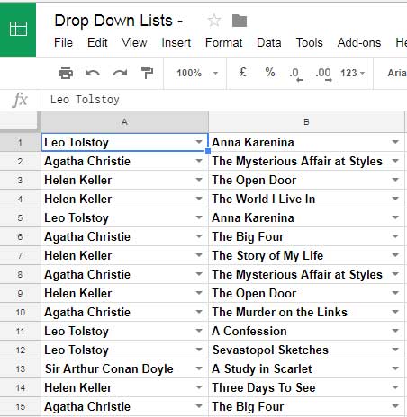
Here in this set of data, column A contains the names of a few of the famous Authors. Here I want to just highlight the names of two authors. For example, here I’m highlighting “Agatha Christie” and “Sir Arthur Conan Doyle”. How to do that?

As I have mentioned, there are two methods – formulas based and without using formula.

Custom Formula to Conditional Format Cells (Multiple Criteria)

Here you can depend on a custom formula that performs an OR logical test. You can tailor the formula in two ways. Any of the below formulas can do this type of conditional formatting.

Formula 1:

=(A1="AGATHA CHRISTIE")+(A1="SIR ARTHUR CONAN DOYLE")

Formula 2:

=OR(A1="AGATHA CHRISTIE",A1="SIR ARTHUR CONAN DOYLE")

To apply this custom conditional formatting rules in Google Sheets, first select the range A1:A10 or whatever the range. Then go to the menu Format and select Conditional Formatting.

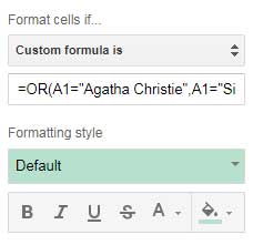
Custom formula for single column multiple condition highlight

Here apply any of the above formulas and choose the color to fill the cells.

This way you can highlight cells based on multiple conditions in Google Sheets. If you want to include more than two conditions, you can simply code the formula as follows.

=(A1="AGATHA CHRISTIE")+(A1="SIR ARTHUR CONAN DOYLE")+(A1="LEO TOLSTOY")

Conditional Format Cells with Built-in Rules (Multiple Criteria)

Same column, multiple criteria conditional formatting is possible without a formula in Google Sheets. In this case, you just need to apply multiple rules as below.

Here I’m highlighting Author’s name in Column A that are matching to “Helen Keller” or “Leo Tolstoy”.

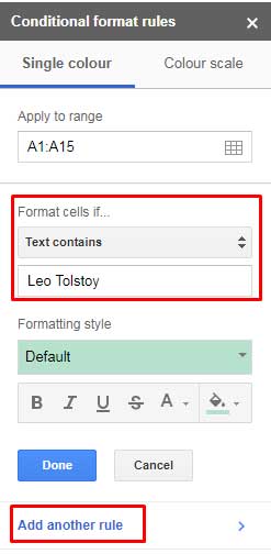
Multiple criteria formatting using format rules

Steps:

Select the range
Go to the Format menu and select Conditional Formatting.
Set the first rule as per the above image.
Click “Add another rule” and add another author’s name.

Highlight a Column Based on Multiple Conditions in Different Columns

The built-in rules are not going to help you here. So you must depend on a custom formula.

For example, here in one column, I have the title of a few books. I want to highlight particular books in that column based on publication date in another column.

Here is my sample data.

Multi column dependent highlighting in google sheets

The content of this data is not accurate. I just filled the names of some random books and fictional publication dates for our example purpose.

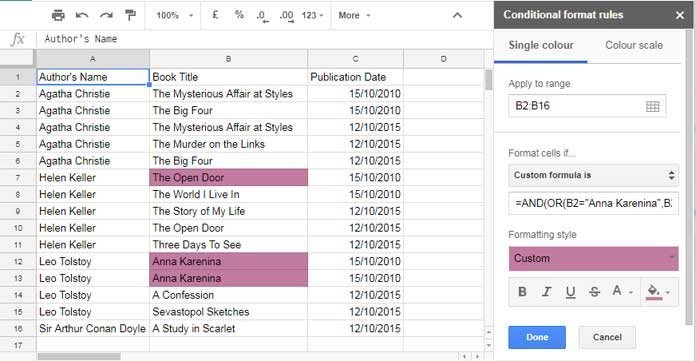
I want to conditional format particular book titles in Column B of which the publication date must be on 15/10/2010. The books are “The Open Door” and “Anna Karenina”. See the publication dates in Column C.

Steps:

Select the column range B2:B16. This’s important. No need to select column C.
You can use the custom below custom formula. It’s AND, OR logical test.

=AND(OR(B2="ANNA KARENINA",B2="THE OPEN DOOR"),C2=DATE(2010,10,15))

This way you can highlight cells based on multiple conditions in Google Sheets. Hope you have enjoyed these tips.

Related Reading:

51 COMMENTS

Paulina J November 11, 2022 At 12:47 am

Hi Prashanth,

Thank you for taking a look.

Here’s an example sheet – I have made it editable. So feel free to play around with it.

– URL removed by Admin –

Currently, the conditional formatting is ok for the green and light pink, but it’s the magenta/darker pink I’m trying to edit.

It’s currently just set to highlight duplicates in col E, but I want to add a condition so that it only highlights the row with the duplicate value in col E and also has a row with a W in col H.

If it’s not doable, then please don’t hesitate to say!

Thanks again!

- Prashanth November 11, 2022 At 1:51 pm
  
  Hi, Paulina J,
  
  Added the formula in your sheet, and the tab name is kvp_test.
  
  You may also like – How to Highlight Conditional Duplicates in Google Sheets.
  
  - Paulina J November 14, 2022 At 3:18 pm
    
    Hi Prashanth!
    
    Amazing! thank you so much for this!
    
    Very grateful for your time and help. All the best.
    
Paulina J November 9, 2022 At 11:57 pm

Hi Prashanth,

Cheers for the post, it’s informative, but I’m still a bit stuck.

Is it possible to add a single formula to look at duplicates in a column, and if there’s a duplicate, highlight the entire row based on whether or not there’s a “W” in Col H?

Happy to make an example if needed.

Cheers.

- Prashanth November 10, 2022 At 12:11 pm
  
  Hi, Paulina J,
  
  Please, feel free to share an example sheet (URL) in your reply.
  
  I won’t publish it.
  
Adam September 1, 2022 At 7:19 pm

Hi,

I have a range of data (A1:D4) containing random numbers.

There is another range in A10:D14, which has another random numbers section.

Question: how can I highlight cells in A1:D4 if numbers match any from A10:D14?

- Prashanth September 2, 2022 At 8:46 am
  
  Hi, Adam,
  
  You can try the below Match formula.
  
  =and(len(A1),match(A1,flatten($A$10:$D$14),0))
  
  Select the range A1:D4 and apply the formula in conditional formatting.
  
  - Adam September 3, 2022 At 3:36 pm
    
    Prashanth,
    
    You are a genius. Thank you so much!
    
John August 7, 2022 At 8:41 am

Hi Prashanth,

Thank you for the great tutorial.

What I am trying to do is if the value of cell A1 is “Promo” and F1 is “Cancelled,” I want the background of A1 to be blue.

I would appreciate it if you have any insight into how I could do this.

- Prashanth August 8, 2022 At 11:27 am
  
  Hi, Johna,
  
  You can use either of the below custom formula rules in cell A1.
  
  Option # 1:
  
  =A1&F1="PromoCancelled"
  
  Option # 2:
  
  =and(A1="Promo",F1="Cancelled")
  
Prashant Kushwah June 14, 2022 At 8:25 pm

Hi Prashanth,

I am a trader in equities.

I am using google sheets in my day-to-day use to track stocks. I stuck up at one point.

My format is something like this below :

Stock — Sector / Industry — Updated date & Time — Mkt. Price — Last Closing — Open — High — Low

I want to highlight the name of the stock, which rises by (let’s say ) 2 % up or down from its open price.

How can I reset my Google sheet to achieve the same?

Regards,

- Prashanth June 15, 2022 At 11:54 am
  
  Hi, Prashant Kushwah,
  
  Please make a sample sheet and include that file’s URL in your reply below.
  
Maria Maria November 30, 2021 At 1:17 am

Hi Prashanth,

I need help. I’m creating a tracker, and it’s a non-numerical value.

Status 1:- My first condition is =$I2="Take Home Assessment" the entire row will be highlighted yellow (this one worked).

But I have another condition. If the candidate failed the Take Home Assessment-

Status 2: =$L2="Unsuccessful" the entire row should turn from yellow to grey.

How can I overwrite the color/highlight of Status 1?

- Prashanth November 30, 2021 At 8:31 am
  
  Hi, Maria Maria,
  
  As you may know, you require to add both the rules. The order of them must be as follows.
  
  Rule 1: =$L2="Unsuccessful"
  Rule 2: =$I2="Take Home Assessment"
  
  Note:- You can drag and drop the rules to change their order.
  
  - Maria Maria November 30, 2021 At 9:34 am
    
    Hi Prashanth,
    
    Glad to hear from you.
    
    Rule 1: =$L2="Unsuccessful" (Grey) – this conditional format works if $I2 is empty.
    
    But if =$I2="Take Home Assessment" is applied, Rule 1 doesn’t work. I can select “Unsuccessful,” but it doesn’t turn the row to Grey 🙁
    
    - Prashanth November 30, 2021 At 11:17 am
      
      Hi, Maria Maria,
      
      The rules work for me.
      
      I think it’s high time to share an example sheet. You can leave the URL below. I won’t publish it.
      
      Thanks.
      
      - Maria Maria November 30, 2021 At 5:30 pm
        
        Hi Prashanth,
        
        Thank you so much for your time and all your help! Thank you.
Amy Smith July 15, 2021 At 6:08 am

Hi Prashanth, thank you so much for your great article!

I’m trying to get column ‘E’ to highlight if columns AC/AE/AG/AG all contain ‘X’ but am struggling, what is the best way to address this? And/OR? IF?

- Prashanth July 15, 2021 At 10:22 am
  
  Hi, Amy Smith,
  
  It’s as simple as this.
  
  Select E2:E, then apply the below rule.
  
  =AC2&AE2&AG2="xxx"
  
  - Amy Smith July 16, 2021 At 3:46 am
    
    Thanks for the reply Prashanth,
    
    I tried inputting that in my google sheets conditional formatting for column ‘E’ as a custom formula and it seems to be highlighting at random and everything but the lines that contain all 4 X in AC/AE/AG/AJ.
    
    - Prashanth July 16, 2021 At 9:52 am
      
      Hi, Amy Smith,
      
      Apply to range: E2:E, not (entire column E)
      
      I haven’t considered column AJ. So, here is the modified formula.
      
      =AC2&AE2&AG2&AJ2="xxxx"
      
      If the above doesn’t help, please share a sample Sheet via comment which won’t be published.
      
Davida July 14, 2021 At 6:30 am

I am wondering if you can help. I want to do something similar to this. From A1:B26, I have a list of criteria. Let’s say in Column A, I have a name, and in column B, I have a color, which can change based on other criteria and formulas I have set up.

From A27:B, I have a list of data points. Let’s say I only want to highlight the data points that match A1 with the color listed in B2.

- Prashanth July 14, 2021 At 4:27 pm
  
  Hi, Davida,
  
  Formula rule for the range A27:Z
  
  =$B27=vlookup("Red",{$B$1:$B$26,$A$1:$A$26},2,0)
  
  Lookup criterion “Red” in B1:B26 and return the name from A1:A26. If that name matches in B27:B, it highlights.
  
  If this doesn’t help, you may share a sample of your sheet.
  
Desmond November 22, 2020 At 12:09 pm

Hi, Prashanth,

I tried your formula above for more than 2 criteria. But it doesn’t seem to work. Don’t know where is my mistake. The formula is;
=AND(OR(H3>8.01,H3 and <12.00 highlight RED. If C1=OUT, Value in H3:AM100 <17.3 highlight RED

- Prashanth November 23, 2020 At 10:59 am
  
  Hi, Desmond,
  
  Thanks for sharing your example sheet. I accessed it and added the below two multiple criteria highlight rules.
  
  RED: If the drop-down in cell C1 has the value “IN”:
  
  =and(H3>8.01,H3<12,$C$1="IN")
  
  ORANGE: If the drop-down in cell C1 has the value "OUT".
  
  =and(len(H3),H3<17.3,$C$1="OUT")
  
  When you change "IN" to "OUT", you may be required to wait a few seconds for the cells to highlight as your sheet is slow responsive due to heavy formulas.
  
Rachyl May 28, 2020 At 10:46 pm

Hello,

I have been trying to put my scenario into sample formulas shown above and cannot figure it out.

I have two columns that contain checkboxes – columns E & H. The text is Red at the beginning for any data entry, and there is a conditional formula coloring a row based on Column C (Last Name).

So, when Column E is checked, I would like it to remove the row coloring. Then, when Column H is checked, I want it to change the text to Black.

So, I can get EITHER of these rules individually but not both at the same time. Can anyone help?

- Prashanth May 29, 2020 At 10:25 am
  
  Hi, Rachyl,
  
  Please leave a sample sheet with EDIT access.
  
  Best,
  
Garrett Fahrbach February 14, 2020 At 8:03 am

Hey there,

I’m messing around with a Google Sheet’s conditional formatting and checkboxes. I’m wanting to change the color of a row based on what checkbox is checked (aka ‘cell’=TRUE).

My range is A2:Y1503. I have my entire first row as a header. I’m using a custom formula and here it is:

=$I2=TRUE

I have columns I:N strictly for checkboxes. I want a row to change to another color if I2 and J2 are checked or only J2 is checked.

What’s the correct formatting for the AND/OR?

- Prashanth February 14, 2020 At 1:59 pm
  
  Hi, Garrett Fahrbach,
  
  Use the below AND/OR formula.
  
  =or(and($I2=TRUE,$J2=TRUE),$J2=TRUE)
  
Harry Jameson January 19, 2020 At 9:03 pm

Hello, I was wondering if it would be possible to highlight a row based on two cells in the row when one of the cells let’s say G hits the same or less quantity as J as a reorder point?

- Prashanth January 20, 2020 At 9:24 am
  
  Hi, Harry Jameson,
  
  Range: A1:Z1000
  
  Formula;
  
  =and(lte($G1,$J1),gt(len($G1)*len($J1),0))
  
  Try this, please.
  
Alexk October 24, 2019 At 7:00 pm

Hi,

I have been looking for days to solve a problem with shading and filtering.

I have a large spreadsheet with all sorts of data in it and I have added a help column to allow me to shade alternate group of rows based on a column’s data using the formula =MOD(IF(ROW()=2,0,IF(D2=D1,J1, J1+1)), 2)

The problem is a need to filter the data all the time losing the alternate shading since the formula still counts hidden rows giving me same shade if the group in between is hidden.

Please help to keep alternate shading grouped by column data regardless of filtering.

I prepared a simplified copy of the spreadsheet in the link below.

Note: Link copied then removed by admin.

Thanks in advance!!

- Prashanth October 25, 2019 At 5:22 pm
  
  Hi, Alex,
  
  I have only a workaround for this problem. I don’t know whether it will suit your needs.
  
  See column K a new helper column on your ‘Product’ tab. Using that column as the criterion, I have filtered the data to a new tab named ‘Product Copy’ and there applied the formatting.
  
  Filter Formula: ={Product!A1:I1;filter(Product!A1:I,Product!K1:K=1)}
  
  Use the ‘Product’ tab for your all kind of filtering. But refer to the helper tab ‘Product Copy’ for the highlighting.
  
  Best,
  
- Prashanth October 26, 2019 At 9:38 pm
  
  Now I have a solution to this problem! I will post it soon.
  
- Prashanth October 28, 2019 At 6:07 pm
  
  Hi, Alexk,
  
  If you are still looking for the solution, try this one.
  
  Alternating Colors for Groups and Filter Issue in Google Sheets.
  
  Best,
  
  - Alexk October 30, 2019 At 8:38 pm
    
    Dear Prashanth,
    
    Although it requires 2 helper columns and 1 helper sheet, it is exactly the result I was looking for! Hopefully, in the future such operations will become integrated into the sheet functionalities as more and more data is needed to be filtered and processed by humans.
    
    I thank you so very much for the solution you found!!
    
    Best Regards,
    
    - Prashanth October 31, 2019 At 8:52 am
      
      Thanks for your feedback!
      
Leah September 4, 2019 At 11:10 pm

Hi,

Hoping for some help with conditional formatting of checkboxes.

Column B is a checkbox for Priority tasks and will highlight the column C task if it is checked. Column D is a Completed checkbox that I am attempting to “strikethrough” column C task if it is checked.

Basically, two different formulas in two different columns affecting a single third column.

I can get them to work independently but if I have one of the checkboxes in column B checked (which causes column corresponding task in column C to be highlighted), then click on the checkbox in column D to indicate that the task is completed, it won’t produce the strikethrough that I need.

Help, please!

- Prashanth September 6, 2019 At 9:18 am
  
  Hi, Leah,
  
  I guess I have correctly interpreted your query.
  
  You have tick boxes in B2:B and D2:D, and the tasks to highlight are in C2:C, right?
  
  You want to highlight the tasks in C2:C in two ways (using tick boxes in two columns).
  
  Conditional Format Rule 1 for the Range C2:C.
  
  =AND(B2=TRUE,D2=TRUE)
  
  Formatting Style: Fill Color & Strike-through.
  
  Conditional Format Rule 2 for the Range C2:C.
  
  =B2=TRUE
  
  Formatting Style: Fill Color.
  
  Please make sure that the highlighting rules are positioned as per my order above. If not it won’t work.
  
Allan August 15, 2019 At 7:38 pm

Can you please help me with my issue?

I trying to do an alternate color formatting. I’ve added a new column (Column D) with values of 1 and 0 (0 change to the grey background while 1 retains a white background).

So far that works, but I need another formatting conditions wherein if Column C is Yes, the entire row will be bolded and change to blue color?

How can I achieve that? Is there a way I can send you screenshot/snapshot so you can better see the issue.

Thanks.

- Allan August 15, 2019 At 8:52 pm
  
  Forgot to mention that the alternating colors apply in every 2 rows.
  
- Prashanth August 16, 2019 At 10:51 am
  
  Hi, Allen,
  
  Instead of sharing a screenshot, please share a demo Sheet. Make an example Sheet and use the Green “Share” button. There click on “Get shareable link”. Then change the settings to “Anyone with the link can edit”. Copy the link and share it in the comment.
  
  I won’t publish the link.
  
  - Allan August 16, 2019 At 7:43 pm
    
    Sure.
    
    - Prashanth August 17, 2019 At 9:38 am
      
      Hi, Allan,
      
      I have added the conditional formatting rules in your Sheet.
      
      Since the Sheet only contains mockup data, I have made a copy of the same and here it is. I hope this can be useful for other users with a similar query.
      
      https://docs.google.com/spreadsheets/d/1NkOG5Xqi_uC2BxTYuOeOn3hoG2171cNXOr5GK2j5-OM/copy
      
      - Allan August 17, 2019 At 6:52 pm
        
        You are a genius. Thank you so much for your help.
      - Prashanth August 18, 2019 At 8:40 am
        
        Welcome!
Tasha Redden July 17, 2019 At 10:41 am

Ok. Scenario – I have a Spreadsheet in Google Drive that I have the conditional format in to change the entire row Blue if it contains a 1 in the Column K. (=$K2="1") – Range is A2:CJ3077 if it matters.

I want to add another layer that says if the number in Column CJ is above 90 then change the color to Red.

Is this possible?

- Prashanth July 17, 2019 At 7:24 pm
  
  Hi, Tasha,
  
  I could understand that the data range is A2:CJ. Follow the below formatting rules.
  
  Red Color (it must the the first rule):
  
  First select this range. In the conditional formatting use the custom formula =and($K2=1,$CJ2>=90). I guess that column A contains the number 1, not the string “1”. If it’s string change the formula as =and($K2="1",$CJ2>=90)
  
  Blue Color (second rule):
  
  Then add one more rule. In that, you can use another custom formula =$K2=1 or =$K2="1"
  
  Best,
  
vaibhav srivastava September 19, 2018 At 12:53 am

It solved my problem! Thanks.

Denise May 18, 2018 At 7:18 pm

Is it possible to highlight cells in column A based on criteria in both column B & C?

- Prashanth May 18, 2018 At 9:41 pm
  
  Hi Denise,
  
  A Custom formula like the one below will highlight all the cells in column A if the values in B=25 and C=30.
  
  =and(B1:B=25,C1:C=30)
  
  You can play around with this formula.