


There is no built-in way to hide formulas in Google Sheets exactly like in Excel. You can either hide the formula bar or follow a workaround.
I am not referring to hiding or unhiding formulas using the keyboard shortcut Ctrl+` (grave accent) which is available in both Excel and Google Sheets. This shortcut toggles the visibility of formulas in the cells.
This keyboard shortcut is useful to copy and paste formulas from Excel to Google Sheets and vice versa. When you copy formulas this way, you can paste the formula itself instead of the value.
Hiding formulas can be useful if you want to prevent others from changing your complex formulas.
When a cell contains a formula, that formula is displayed in the formula bar when the cell is selected. However, if you don’t want to display formulas for any reason, you can easily hide them in Excel.
In Google Sheets, you can’t hide formulas, but you can replace them with an imported result. Ultimately, your complex formula will be safe in another file.
How to Hide Formulas in Excel
This method hides the formulas in the selected cells and password-protects them, so that, only users with the password can view and edit them. The other cells in the sheet will still be available for editing.
Steps:
Select all cells by clicking the Select All button (please see Figure 1 below).
On the Home tab, in the Cells group, click Format > Format Cells.
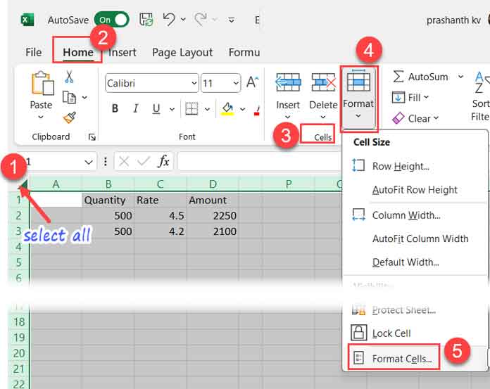
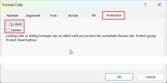
In the Protection tab, uncheck the Locked checkbox and the Hidden checkbox. Then, click OK.
Select the cells that contain the formulas you want to hide. You can use Shift+click or Ctrl+click to select multiple cells.
In the Format Cells dialog box (please see Figures 1 and 2 above), go to the Protection tab, check the Locked and Hidden checkboxes, and click OK.
On the Review tab, in the Protect group, click Protect Sheet.
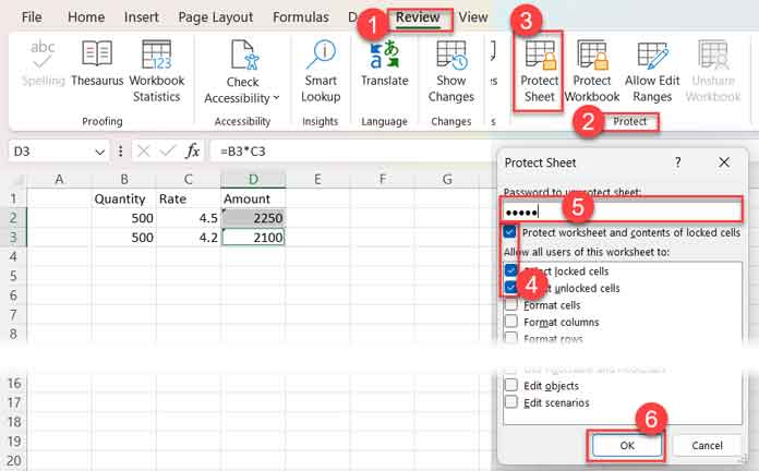
Tick the checkboxes, if already not, that correspond to the following:
- Protect worksheet and contents of locked cells.
- Select locked cells.
- Select unlocked cells.
Enter a password, click OK, then enter the password again to confirm, and click OK.
2 Easy Ways to Hide Formulas in Google Sheets
Google Sheets does not have an option to hide formulas natively, unlike Excel. Here are two workarounds:
- Hide the formula bar. This will prevent users from seeing the formulas in the cells, but they will still be able to see the results of the formulas.
- Replace the formula with an IMPORTRANGE formula. This will create a link to another sheet that contains the formula. When the formula is calculated, the results will be pulled from the other sheet.
How to Hide the Formula Bar in Google Sheets
You can hide or unhide the formula bar in Google Sheets from the View menu. Click View and select Show > Formula bar.
Use this method if the formula bar distracts you. You can still see the formula within the cell by double-clicking it.
Using IMPORTRANGE Function to Hide Formulas in Google Sheets
Using the IMPORTRANGE function is another way to hide formulas in Google Sheets. In this method, we will replace the original formula with an IMPORTRANGE formula.
The IMPORTRANGE function imports data from another sheet and updates the imported data whenever the source data changes.
We can adopt a two-way import to hide formulas in Google Sheets. This involves importing the source data to a second file, processing the data (applying the formula) there, and then importing the processed data (formula result) back.
Steps
Open the sheet in which you want to hide the formulas. For example, let’s consider the following sheet. The file name is “Schedule” and the tab name is “Sheet26”.

There is a very complex formula in cell C4 that checks the dates in column A and marks the dates that correspond to the payment period selected in cell B1 and the start date in cell B2.
The formula returns the results in column C as it is an array formula. I want to hide this formula due to proprietary reasons.
Note: If you are following my example, you can use a basic array formula in cell C4 for testing purposes, such as:
=ARRAYFORMULA(TEXT(A4:A,"DDD"))First, we need to make a copy of this file. We can do that from the File menu > Make a copy.
In the copied sheet named “Copy of Schedule,” remove everything except the formula in cell C4.
In cell A1, use the following formula to import the data from columns A and B from the “Schedule” file:
=IMPORTRANGE("paste_Schedule_file_url_here","Sheet26!A1:B")Syntax of the IMPORTRANGE Function in Google Sheets:
IMPORTRANGE(spreadsheet_url, range_string)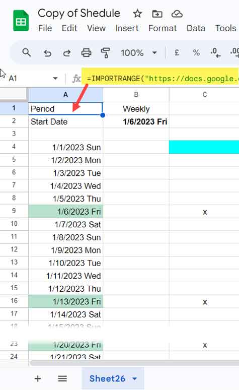
In the “Schedule” file, in cell C1, insert the following IMPORTRANGE formula:
=IMPORTRANGE("paste_Copy_of_Schedule_file_url_here","Sheet26!C1:C")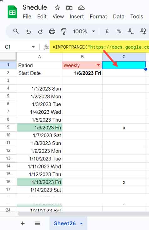
Finally, do one more thing. Make sure that the file sharing settings of the “Copy of Schedule” file are set to “Restricted.” If you are unfamiliar with this setting, you can check my guide Sharing Google Sheets Files in Copy Mode. Then close this file.
Now you can work in the “Schedule” file as usual. Your changes in columns A and B (formula range) will be reflected in the formula result in column C. However, it may take some time for the changes to be processed because of the two-way import.
I have made updates to the solution.
How can do the same process for a chart on its own sheet? Do I link the chart data series the same way?
There is a very easy solution for people accessing WITHOUT being logged into a Gmail account.
In your main sheet, copy and paste all content from Sheet1 into a new page. Name it “Formulas” (or something sensible).
Delete all the formula cells in the main sheet. This will now be referred to as Input page.
* In your Input page, call upon all formulas from Formulas page.
* In your Formulas page, call upon all input fields from Input page.
* Hide (right click) Formulas page and Hide it.
Share, set permissions, tick privacy settings, send an invite.
Then, then the only way for Gmail users to view the code is to go View -> Hidden Sheets.
However, if not logged into using Gmail, this function is hidden and there’s no way to access Formulas page.
Very annoying that you cant set permissions on hidden pages.
What’s the point I did it, it works, but then the linked sheet has no functionality it just a view/mirroring the original.
What if I want users that I’m sharing the mirrored version to enter data that affects the formulas calculations???
That’s a limitation 🙁
Hey,
Great article.
I had a small doubt,
I have created a stock tracker in Google finance and I don’t want to share the formula sheet.
So I did the following steps,
But now the live feed is not working in the importance sheet.
Any suggestions
It works! It’s a little slow, but that’s ok. Thank you!
I was finally able to get IMPORTRANGE to fetch data. However, my goal was to let others edit 2 other cells on the spreadsheet. It seems this won’t work. The cells that contain IMPORTRANGE will not work. The values stay the same.
Hi Mike,
I can understand.
I hope this can solve your issue. But the problem is, it can slowdown the process. That is why, I limited my tutorial to that extend.
See that there is now two importrange formulas, one in each file.
Thanks,
Prashanth
I used this and it still did not work:
=IMPORTRANGE("https://docs…./d/1Ow..gid=xxxxxxxxx","Sheet1!E5:G9")I wasn’t sure where to find the name of the sheet, so I used Sheet1. It looks like it is not working for other people.
Hi,
Please note that sheet name is the Google Sheets Tab Name. You should use this correctly.
Prashanth
Thanks for your reply. I just tried it again with the same IMPORTRANGE function and it gives me this message — Error Cannot find range or sheet for imported range. I have seen the allow access message but when I clicked on it, it didn’t work. I currently have the privacy set so only I can access Master1. I’m not sure what I could be doing wrong. Any ideas?
Hi,
It works like this.
You have one file named as “File A”. You want to hide formula in this.
Make copy of file A. We can name this as “Copy of File A”. Set this file Private.
Come back to File A and delete the formulas you want to hide. Then use import range function to import the content from “Copy of File A”. Inside the importrange function use the entire URL of “Copy of File A” as it is and use the sheet name and range. All within quotes as per our tutorial.
If you get that error means, your importrange formula is wrong.
Please cross check.
Thanks.
I created a spreadsheet with range A1:G9 and named it “Master.” Then I clicked on file/make a copy, and named the copy “Master Copy.” I right-clicked on “Master Copy” in Google drive and it was already set to off-specific people.
I go back to “Master Copy” and delete range E5:G9. I replace that range with
=IMPORTRANGE("https://docs..../d/1Ow..gid=xxxxxxxxx","SHEET1!E5:G9")It gives me #REF! In cell E5. In the IMPORTRANGE function, I used the nine numbers corresponding to my gid=xxxxxxxxx. I assumed I was not supposed to put gid=0. I was not sure where you got SHEET1 from.
I keep trying to figure this out but I’m not sure where I am making a mistake. Can you please help?
Hi,
You did everything correctly. You will, of course, get that error!
Just point your cursor at the error. You can see a message popup to “Allow Access.”
Click on it and allow access. That’s all.
I should have mentioned it in the tutorial. I will add that part to the tutorial too.
Cheers!
I tried to do this but was not successful. Are you still able to do this? I could’ve easily done something wrong as I’m not proficient at working with Google sheets.
Hi Mike,
I have two sections on this post. One is dealing with Excel and other with Google Sheets. You may please check the steps under the title “Excel Alternative to Hide Formulas in Google Sheets Formula Bar”. It will definitely work.
Regards,
=importrange is not working , I have done same as you said, error only
Hi Ramesh,
Can you share me more details. If possible a sample sheet with edit access.
Prashanth
Your sheet maybe in xlsx format, convert it into Google Sheets.