I am sure that our topic discussing Google Sheets Query hidden row handling is new to you.

You can select only visible rows using the QUERY function in Google Sheets.

That means when you use a Query formula to an already filtered data (or data containing hidden rows), it will only pull the visible rows. It is not possible in the usual case!

Here, with this tutorial, you can learn how to add this powerful feature to a Query formula using a workaround approach.

For this purpose, we will use a virtual helper column (an additional column that is not physically available in the dataset).

Hidden rows are a nightmare for many spreadsheet users as it invites unwanted results.

Several powerful functions, such as SUMIF, Query, and SUMPRODUCT, fell short of handling hidden or filtered-out rows.

The only possible way to deal with hidden rows is by using the SUBTOTAL function and associated function numbers.

But the Subtotal function has a limitation. It doesn’t accept conditions or expand down automatically with an ARRAYFORMULA.

With our virtual helper column concept, you can overcome some of the Query hidden rows handling related dilemmas. So here we go.

Google Sheets Query Hidden Row Handling and Virtual Helper Column

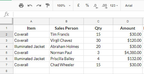
Here is the sample data.

It contains item names, names of the salespersons, sales quantity, and sales amount in columns A, B, C, and D, respectively.

We will hide 2-3 rows and see how to omit that rows while manipulating this data using the Query function.

Usually, it is not possible to select only visible rows using Query. But with our virtual helper column concept, we can do it.

So here are the steps to create that virtual helper column in Google Sheets.

How to Create a Virtual Helper Column for Query to Select Only Visible Rows

There are two methods.

I don’t recommend approach # 1 below, as it’s no more exciting after the launch of the Byrow function in Google Sheets.

So please scroll down and follow approach # 2.

Approach # 1 (Old Method)

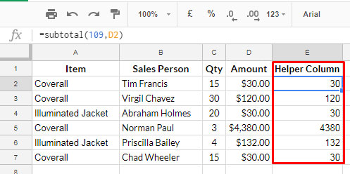
Let’s add a new column at the end of the data called a helper column. 

Of course, we will delete this physical helper column later on.

We have the following Subtotal formula in E2, which we must copy-paste down the column.

=subtotal(109,D2)

When you use this formula, you must choose any numeric field.

Replace Subtotal(109, with Subtotal(103, in case you don’t have a numeric column.

But make sure that there are no blank cells in the referred column range here D2:D7.

Here is the second step to Query hidden row handling.

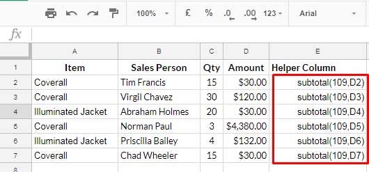
Go to the menu View > Show formula.

Then remove all the “=” sign prefixes in the subtotal, and it must look like the below E2:E7 range.

Again go to the View menu and click on Show Formula to remove the selection.

Apply the below formula in any blank cell outside the above range to join all the strings in column E.

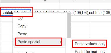
=join(";",E2:E7)

It returns the combined texts in column E. You may copy the formula result, right-click on the cell, and then apply the paste value.

Add Curly Brackets at the beginning and end of the string as below. Your virtual helper column is ready!

{subtotal(109,D2);subtotal(109,D3);subtotal(109,D4);subtotal(109,D5);subtotal(109,D6);subtotal(109,D7)}

Now you can delete the helper column E. Now we have a long text to use as a virtual helper column for Query.

Approach # 2 (New Method)

In approach # 1, we have copy-pasted the E2 formula, i.e., =subtotal(109,D2), down, edited and combined to handle hidden rows in Query.

Now that is not required as we can automatically expand the E2 formula down using BYROW as below in E2.

=byrow(D2:D7,lambda(r,subtotal(109,r)))

If you specify any text range (field) instead of the numeric range D2:D7, use function number 103 within the Subtotal.

Join Virtual Helper Column with Query and Hidden Row Handling

Let me apply a simple Query formula to select only visible rows from our sample data above.

Beforehand, you may hide one or two rows using the Data menu Filter or right-click and manually hide any two rows.

First, see the usual Query formula, which will pull all the data from the source, including the hidden rows.

=query({A2:D7},"Select Col1, Col2, Col3, Col4")

Now see our new Query formula with the virtual helper column below.

As Per Approach # 1:

=query({A2:D7,{subtotal(109,D2);subtotal(109,D3);subtotal(109,D4);subtotal(109,D5);subtotal(109,D6);subtotal(109,D7)}},"select Col1, Col2, Col3, Col4 where Col5>0")

As per Approach # 2: Recommended

=query({A2:D7,byrow(D2:D7,lambda(r,subtotal(109,r)))},"select Col1,Col2,Col3,Col4 where Col5>0")

You May Like: What is the Correct Clause Order in Google Sheets Query?

We have four columns in our sample data. Column 5 is our virtual helper column.

When we hide any rows, the value in the virtual helper column corresponding to that row becomes zero.

So it will be automatically excluded from the Query output due to our “Where” clause condition, i.e., where Col5>0, in Query.

I hope you have enjoyed this tutorial and learned the Google Sheets Query Hidden Row Handling feature/workaround.

See you again with another spreadsheet tutorial.

Sample_Sheet_171220