


The advantage of the Google Sheets MAXIFS function lies in its ability for multiple condition filtering, distinguishing it from MAX or LARGE.
When you need to retrieve the maximum value in a range of cells filtered by specific criteria, the Google Sheets MAXIFS function proves reliable. However, if you aim to obtain not only the maximum value but also another value from the same row, it is preferable to use FILTER or QUERY.
In this tutorial, we will delve into applying the MAXIFS formula in Google Sheets.
MAXIFS Function: Syntax and Arguments
Syntax:
MAXIFS(range, criteria_range1, criterion1, [criteria_range2, criterion2, …])Arguments:
In the MAXIFS function, the first three are the required arguments, and others are optional. Let’s take a quick look at the arguments in this function.
range: The range for which you want to find the maximum value. It should be a physical range, not an expression, such as an IMPORTRANGE formula.criteria_range1: The criteria range of the same size as therange.criterion1: The pattern or test to apply tocriteria_range1.criteria_range2,criterion2, … (Optional): Additional criteria ranges and their associated criteria.
Sample Data
To thoroughly test the MAXIFS function with various scenarios, including:
- MAXIFS with a single criterion.
- MAXIFS with multiple criteria:
- Using multiple criteria in the same column (OR).
- Using multiple criteria in multiple columns (AND).
I’ve prepared a sample table below for your testing purposes. Copy and paste it into cells A1:D10 on your sheet to evaluate the provided formulas.
| Name | Score | Attempts | Remarks |
| Alice | 800 | Attempt 1 | |
| Bob | 900 | Attempt 1 | |
| Charlie | 850 | Attempt 1 | |
| Alice | 850 | Attempt 2 | |
| Bob | 950 | Attempt 2 | |
| Charlie | 800 | Attempt 2 | |
| Alice | 800 | Attempt 3 | |
| Bob | 900 | Attempt 3 | Failed |
| Charlie | 1000 | Attempt 3 |
Now, let’s move on to the example formulas.
Using MAXIFS Function with Single Criterion
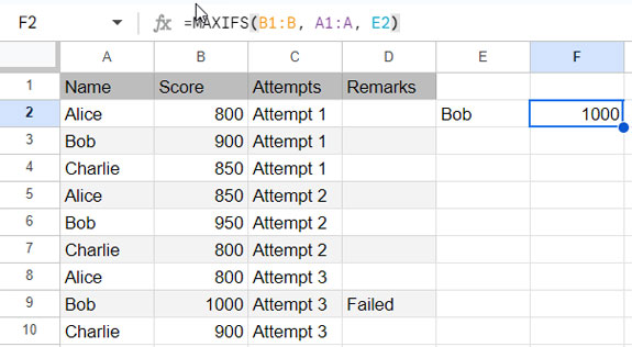
To find the maximum score of Bob, you can use the following formula:
=MAXIFS(B1:B, A1:A, "Bob")Where:
- B1:B is the
range. - A1:A is the
criteria_range1. - “Bob” is the
criterion1.
The formula will return 1000, which is the maximum score of Bob.
The following screenshot illustrates the usage of the MAXIFS function in Google Sheets.
Using MAXIFS Function with Multiple Criteria (AND Logic)
In the previous example, we utilized only one criteria range and one criterion.
Now, let’s explore using two criteria ranges and two criteria, one from each criteria range. This is referred to as multiple criteria AND in MAXIFS in Google Sheets.
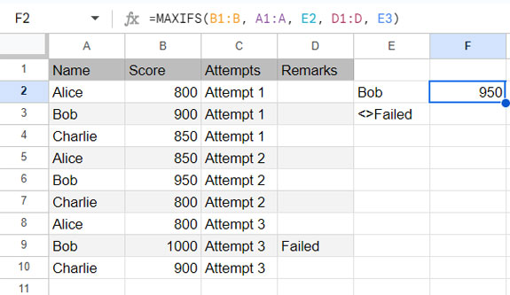
How do we find the maximum score of Bob excluding the failed attempt score?
=MAXIFS(B1:B, A1:A, "Bob", D1:D, "<>Failed")The above formula returns the maximum score in B1:B for “Bob” in A1:A, excluding any scores with “Failed” in D1:D. The result would be 950.
Using MAXIFS Function with Multiple Criteria (OR Logic)
How do we implement OR logic in MAXIFS in Google Sheets?
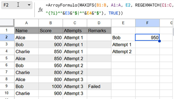
When testing multiple criteria in the same column, such as finding the maximum score of Bob in the first and second attempts or excluding the third attempt, we need to apply OR logic in MAXIFS.
To achieve this, you can use the REGEXMATCH function within MAXIFS. This is necessary because MAXIFS alone cannot handle testing multiple criteria in the same column.
The REGEXMATCH function tests multiple criteria and returns TRUE or FALSE. We will use TRUE as the criterion and the REGEXMATCH formula as the range to test.
So, ultimately, the issue of multiple criteria or logic doesn’t apply. Here is the formula:
=ArrayFormula(MAXIFS(B1:B, A1:A, "Bob", REGEXMATCH(C1:C, "(?i)^Attempt 1$|^Attempt 2$"), TRUE))The ARRAYFORMULA is used to populate an array result in REGEXMATCH.
In this formula:
- B1:B is the
range. - A1:A is
criteria_range1. - “Bob” is
criterion1. REGEXMATCH(C1:C, "(?i)^Attempt 1$|^Attempt 2$")iscriteria_range2. (Removing the anchors^and$allows for a partial match of the criterion.)- TRUE is
criterion2.
In REGEXMATCH, C1:C is the range to match, and "(?i)^Attempt 1$|^Attempt 2$" is the regular expression to match.
Additional Notes
Here are a few tips for using criteria in the MAXIFS function.
- Use double quotes for text criteria when entering the criterion directly into the MAXIFS formula, e.g.
"Apple". - Enter numbers without double quotes for numerical criteria, e.g.,
10.50. - Represent dates using the DATE function with the syntax
DATE(year, month, day). - Express time using the TIME function with the syntax
TIME(hour, minute, second). - Combine date and time as a timestamp using the syntax
DATE(year, month, day)+TIME(hour, minute, second). - For a tutorial on partial matching of criteria, refer to: Three Main Wildcard Characters in Google Sheets Formulas.
It is advisable to input the criterion within a cell and refer to that cell in the MAXIFS, ensuring that you don’t need to worry about remembering the specific syntax.
Regarding the comparison operator usage, see an example under MAXIFS AND logic above.
Can we use multiple column ranges in the Google Sheets MAXIFS function?
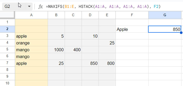
Yes! Let’s assume you have fruit names in column A and their quantities scattered in columns B to E. Now, let’s find the maximum quantity of Apple.
To achieve this, count the number of columns in the range (B to E) which is 4. Replicate the range 4 times as follows in criteria_range1:
=MAXIFS(B1:E, HSTACK(A1:A, A1:A, A1:A, A1:A), "Apple")This formula will return the maximum value in the range B1:E if for “Apple” in A1:A.
That’s about using MAXIFS in Google Sheets. Thanks for staying. Enjoy!
Related: Master MAXIFS Array Formulas in Google Sheets: The Ultimate Guide.
What if the data ranges are in another sheet than the current one?
E.g.:- Sheet 1 contains the formula, and sheet2 contains the data.
What if you want to do another operator than OR?
For instance, the condition should contain Germany. So both east and west Germany count.
And the upper/lower case of the country shouldn’t matter.
Hi, Nico,
If Sheet2 contains the data, include that in the range and criteria range.
=maxifs(Sheet2!H4:H,Sheet2!C4:C,"Germany")Regarding your second question, use wildcards.
=maxifs(Sheet2!H4:H,Sheet2!C4:C,"*Germany*")It’s a case-insensitive formula.
And here is an equivalent formula.
=ArrayFormula(MAXIFS(Sheet2!H4:H,regexmatch(Sheet2!C4:C,"(?i)germany"),TRUE))In this last MAXIFS formula, remove
(?i)to make it a case-sensitive formula.