


The INDIRECT function in Google Sheets returns a cell, range, or named range reference specified by a string. It’s particularly useful for dynamic referencing and in conditional formatting across multiple sheets.
When you use regular cell references like A1:C10 or $A$1:$C$10, inserting rows or columns can cause these ranges to shrink or expand unexpectedly. By employing the INDIRECT function, you can refer to ranges more flexibly.
Understanding the INDIRECT function in Google Sheets is crucial for managing and manipulating data effectively, especially when dealing with dynamic data or complex formulas.
Syntax
INDIRECT(cell_reference_as_string, [is_A1_notation])cell_reference_as_string: A cell, range, or named reference specified as a string with surrounding quotation marks. Examples include “A1”, “C10:E20”, or “sales”.is_A1_notation: An optional argument indicating whether the cell reference is in A1 (default) or R1C1 notation. Specify TRUE or FALSE. If omitted, the function will default to A1 notation.
Google Sheets primarily utilizes A1 notation, where cells are addressed by their column letter and row number (e.g., A1, B2). There is no setting to switch to R1C1 notation within Google Sheets.
In R1C1 notation, cells are referenced by their row and column numbers. Here are a few examples:
- R1C1 (row #1 and column #1) refers to cell A1.
- R5C26 (row #5 and column #26) refers to cell Z5.
- R1C1:R5C26 refers to the cell range A1:Z5.
In R1C1 notation, the number in square brackets indicates the relative position from the current cell. For instance, if the current cell is H10, R[0]C[-1] refers to cell G10.
INDIRECT Function: Formula Examples
In the INDIRECT function, we can specify cell_reference_as_string in two ways: as a cell reference and hardcoded (directly within the formula).
We will start with hardcoding.
cell_reference_as_string: Hardcoded
Example 1:
=INDIRECT("A1") // returns the cell reference A1
=INDIRECT("R1C1", FALSE) //  equivalent
Example 2:
=INDIRECT("A3:D4") // returns the range reference A3:D4
=INDIRECT("R3C1:R4C4", FALSE) // equivalent
As per the above examples, you can understand one thing. If you want to sum the range A1:C100, you can use =SUM(INDIRECT("A1:C100")).
Do you know when these types of hardcoded cell_reference_as_string are useful in the INDIRECT function in Google Sheets?
Assume you want to sum the range B2:2 (the entire second row from column 2). If you use =SUM(B2:2) in cell A2, the range will become C2:2 if you insert a column immediately after A. But if you use =SUM(INDIRECT("B2:2")), the reference won’t change as it’s a string. This ensures that the formula always returns the sums of the range from the second column to the last column in the sheet.
Note: Using R1C1 notation may make your formulas complex, so I suggest sticking with A1 notation.
cell_reference_as_string: Strings in Cells
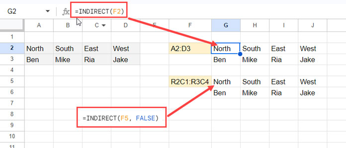
Instead of hardcoding the cell_reference_as_string within the formula, you can enter it into a cell and then refer to that cell within the INDIRECT function. Please see the screenshot for the examples.
Formulas:
=INDIRECT(F2) // formula in cell G2
=INDIRECT(F5, FALSE) // alternative formulain cell G5
Cell F2 and F5 contain A2:D3 and R2C1:R3C4, respectively (they should not be entered within double quotation marks).
INDIRECT a Different Sheet in Google Sheets
To INDIRECT a different sheet, include the sheet name followed by an exclamation mark with the cell reference.
For example, =INDIRECT("Sheet1!A1") will return the value of cell A1 in Sheet1.
The above represents the hardcoded way of using cell_reference_as_string. Alternatively, you can enter the sheet name with or without the cell reference in a cell and refer to that.
=INDIRECT(F10&"!A1") // when cell F10 contains "Sheet1"
=INDIRECT(F10) // when cell F10 contains "Sheet1!A1"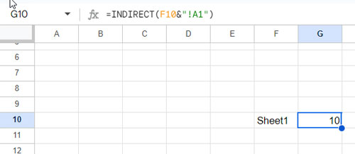
Note: You must use an INDIRECT range when referring to a different sheet in a custom formula rule in conditional formatting. Otherwise, the sheet will return “Invalid range” or display the following message: “Conditional format rule cannot reference a different sheet.” This doesn’t apply to data validation rules.
INDIRECT Function with Named Ranges in Google Sheets
If you name a range A1:A10 as “employee,” you can refer to it using either =ArrayFormula(employee) or =INDIRECT("employee"). The named range should be entered as a string within the INDIRECT function, and using ArrayFormula isn’t necessary.
However, typically, we don’t use indirect named ranges in this manner. They are usually employed to create dynamic ranges.
Let’s create a dynamic named range using INDIRECT and XMATCH functions in Google Sheets.
Assume you want to refer to the range between two lookup values in column A dynamically. Here’s how you can do it:
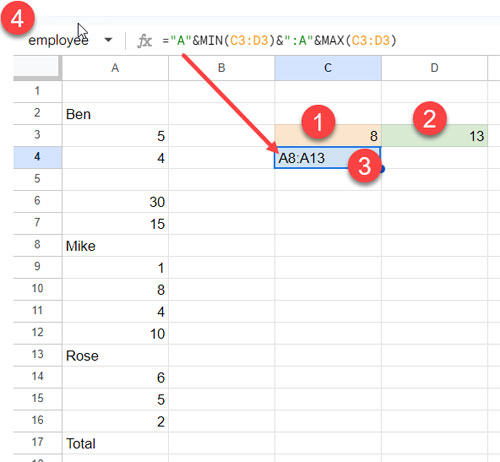
For example, =XMATCH("Mike", A:A) and =XMATCH("Rose", A:A) will return the positions of “Mike” and “Rose” in column A.
Enter these formulas in cells C3 and D3, respectively.
In cell C4, enter the following formula to return a range reference string:
="A"&MIN(C3:D3)&":A"&MAX(C3:D3)Navigate to cell C4 and enter the name “employee” in the “Name box” located to the left of the formula bar.
Then, try the following formula in cell D4 after clearing D4:D:
=ArrayFormula(INDIRECT(employee))When you modify the lookup values in the XLOOKUPs, the formula in cell D4 will refresh the result accordingly.
Resources
The main drawback of Google Sheets INDIRECT function is its inability to refer to multiple indirect ranges from cells. We can’t use it like =INDIRECT(A1:A2) where A1 and A2 contain cell references or range reference strings. However, we can use LAMBDA helper functions (LHFs), especially REDUCE, to solve this.
Here are some Google Sheets tutorials where you will find advanced uses of the INDIRECT function, including the REDUCE LHF:
- Role of Indirect Function in Conditional Formatting in Google Sheets
- Highlight Indirect Range in Google Sheets
- Alternatives to INDIRECT with ArrayFormula in Google Sheets (Using LHFs)
- Dynamic H&V Named Range in Google Sheets
- Combine Data Dynamically in Multiple Tabs Vertically in Google Sheets
- Dynamically Combine Multiple Sheets Horizontally in Google Sheets
Hello,
I am searching for a formula that includes the INDIRECT function in the QUERY function because my data is on multiple sheets.
Thank you.
Hi, Arun Kumar Gupta,
It won’t work the way you want. I have included the workaround in the following tutorial – How to Include Future Sheets in Formulas in Sheets.
OMG, this changed my life forever!
Thank you so so much!
Thank you so much!
Your answer works perfectly. I spent so many hours trying to research this, you saved me a ton of time and I can’t thank you enough! I have bookmarked this site and will be coming back to read all the articles about sheets.
Again, thank you!
Hello,
I have been searching for an answer to an error I have come across and after reading many articles and reference items I was hoping you might be able to help me.
I am trying to count the blank rows in a dynamic and partially filled column. I have a reference to the last filled Row at:
'Formula Ref'!B3In another tab I am trying to reference the number in this cell to use as my end point to a range for the countblank function. No matter what I try I always get 0 as the answer when I know that the range I am searching has 276 blank cells. I am trying with this formula:
=COUNTBLANK('Data - Sanatized'!H1:Indirect("H"&'Formula Ref'!B3))This works fine if I am not referencing a separate sheet in the opening part of my formula:
=COUNTBLANK(H1:Indirect("H"&'Formula Ref'!B2))The above works correctly on the current sheet but when I try and make it reference the data sheet it fails to count.
Any help would be GREATLY appreciated.
Hi, Jason,
Here is the correct Indirect formula when you want to refer to a different sheet.
=countblank(indirect("'Data – Sanatized'!H1:"&"H"&'Formula Ref'!B3))Error!
Hi, SPH,
Please see this.
Hi,
This formula gives an error.
=arrayformula(HistoricalMM!INDIRECT(H1):BN)H1 = “BN”.
BN dynamically changes. I want the latest.
This works:
=arrayformula(HistoricalMM!BN:BN)Thanks
Hi, SPH,
Try this Indirect formula.
=indirect("HistoricalMM!"&H1&":BN")Hi there, I am stumped on a Google sheet problem and have read tons of blogs without any avail. It seems to me that it would be simple, but I haven’t found the right formula yet.
What I am attempting to do is yield a sum value based on three criteria. However, the criteria changes per row. I’ve made it work generally with an array formula
=ArrayFormula(sumif('Expense Tracker (NEW)'!$B$4:$B$150&'Expense Tracker (NEW)'!$D$4:$D$150&'Expense Tracker (NEW)'!$E$4:$E$150,"Jan"&"Operational"&"Mortgage ",'Expense Tracker (NEW)'!$K$4:$K$150))but I would rather the criteria indicators
"Jan"&"Operational"&"Mortgage "be conditional on the value of a given cell vs. the exact text.This is for a financial tracking sheet where I input an expense in one tab (Expense Tracker (NEW)) and then categorize the expense using by selecting the date, type of expense (operational or project), and expense category.
The intent is that on the second tab the formula will summarize the sum of values in the expense tracker depending if the month matches and the expense line item.
Here is the link to the sheet I am working on: … link removed by admin …
Any help or advice would be sincerely appreciated!
Hi, Cydney,
No need to use INDIRECT in the formula. Also, when there are multiple conditions to consider in the SUM, the recommended function in your case is SUMIFS.
Please see the new tab in your sheet named “info inspired”.
I have inserted the below SUMIFS in P25 which then copied to its right and down.
=sumifs('Expense Tracker (NEW)'!$K$4:$K,'Expense Tracker (NEW)'!$B$4:$B,P$4,'Expense Tracker (NEW)'!$D$4:$D,"Operational",'Expense Tracker (NEW)'!$E$4:$E,$A25)I hope, this helps.
Hi, Cydney,
I think you are looking for an array formula. Then use the below SUMIF.
=ArrayFormula(sumif('Expense Tracker (NEW)'!B4:B&'Expense Tracker (NEW)'!D4:D&'Expense Tracker (NEW)'!E4:E,P4:AA4&"Operational"&A25:A43,'Expense Tracker (NEW)'!K4:K))The same you can find in cell P24 in “info inspired 2”
OK. I have figured it out. Thanks a lot to you, you solved it.
Thank you very much.
I used the formula and this is what I experienced.
When I paste it in K10, it gives #ref error. It works when I paste it in B10. But it is K10 (E10, H10, and so on) where it needs to work.
Thanks.
Sorry, I did not get any notification that you have posted.
The formula that I use is copied from an article of yours. The link to my spreadsheet is – link removed by admin –
I give comments in I, J, K2 merged columns.
Thanks
Hi, SPH,
No issue 🙂
In my old posts, I have used RANDBETWEEN to shuffle rows.
Now after the introduction of RANDARRAY, we can use an even shorter formula to randomize the range J10:J23 (we can make the range dynamic using the Indirect function later).
=sort(J10:J23,randarray(14,1),0)Here is the more flexible version of the above same formula and we will use it.
=sort(J10:J23,randarray(rows(J10:J23),1),0)Now the question is how to use Indirect to dynamically use the range J10:J23.
The following formula in any column in row # 10 would return the range J10:J23 in text format (the active row number and the row number of the last value in column J).
=address(row(),column(J1),4)&":"&SUBSTITUTE(ADDRESS(1,column(J1),4),1,"")&
ArrayFormula(MATCH(2,1/(J:J<>""),1))
Wrap this formula with Indirect and replace the range J10:J23 in the
=sort(J10:J23,randarray(rows(J10:J23),1),0)formula twice.Here is the formula after the said modifications.
=sort(indirect(ADDRESS(row(),column(J1),4)&":"&SUBSTITUTE(ADDRESS(1,column(J1),4),1,"")&ArrayFormula(MATCH(2,1/(J:J<>""),1))),
randarray(rows(indirect(ADDRESS(row(),column(J1),4)&":"&
SUBSTITUTE(ADDRESS(1,column(J1),4),1,"")&ArrayFormula(MATCH(2,1/(J:J<>"")
,1)))),1),0)
You can feel free to remove the two ArrayFormulas and their corresponding open and close brackets from the above formula.
Now you can use Index, Array_Constrain, Sortn, or Query to limit the output to 1. I’m using a Query.
=query(sort(indirect(ADDRESS(row(),column(J1),4)&":"&SUBSTITUTE(ADDRESS(1,column(J1),4),1,"")&MATCH(2,1/(J:J<>""),1)),
randarray(rows(indirect(ADDRESS(row(),column(J1),4)&":"&
SUBSTITUTE(ADDRESS(1,column(J1),4),1,"")&MATCH(2,1/(J:J<>""),1))),1),0),
"Select * where Col1 is not null limit "&indirect(K7))
See if this helps?
Hi, SPH,
It’s because the cell J9 in which you have an Indirect. Before my formula, that cell was returning blank and so I was unaware of it. After my formula in cell K10 it (cell J9 formula) returns a circular dependency error. I tested my formula in cell L10 so I haven’t notice that.
Whenever you ask questions, the better practice is just to provide a demo sheet without any formulas. You have several formulas all over your sheet. It’s not possible for me to go through all the formulas.
Thanks for your understanding.
Hi,
I use the following formula in google sheets.
=ArrayFormula(Array_Constrain(vlookup(Query({ROW(D8:D23),randbetween(row(D8:D23)^0,9^9)},"Select Col1 order by Col2 Asc"),{row(D8:D23),
D8:D23},2,FALSE),$D$3,1))
I wish to replace
d8:d23withd8:indirect(a4). Normallyindirect(a4)works, but in this case it gives an error.Each column has a different no. of filled rows and the formula has to adjust dynamically else I get a few blanks in my output when I use a fixed range.
Thanks
Hi, SPH,
It seems, your ArrayFormula without Indirect itself is not correct!
This part is OK.
Query({ROW(D8:D23),randbetween(row(D8:D23)^0,9^9)},"Select Col1 order by Col2 Asc")The Vlookup seems not as per the syntax.
vlookup(Query({ROW(D8:D23),randbetween(row(D8:D23)^0,9^9)},"Select Col1 order by Col2 Asc"),{row(D8:D23),D8:D23},2,FALSE)If you explain the purpose of your formula or share with me an example sheet, then I may be able to help you with the formula and the Indirect function usage too.