How to Utilise Google Sheets Date Functions [Complete Guide]

This tutorial about utilizing Google Sheets date functions is divided into three subcategories for easy explanation – Simple Date Functions, Standard Date Functions, and Advanced Date Functions.

I have spent lots of my time writing tutorials related to Google Sheets’ advanced functions, charts, and other important aspects related to Google Sheets.

As a result, you can see plenty of tutorials related to Google Sheets on this Site. So what’s the point?

The thing is that I intentionally opted out of writing some of the commonly used Google Sheets functions that I thought users might know. The Google Sheets Date functions are one among them.

In order to make Info Inspired a complete reference source for Google Sheets users, I am filling that void space with the so-called ‘missing’ functions.

So here we are. Let us begin with how to utilize Google Sheets Date functions.

Simple Google Sheets Date Functions

Google Sheets TODAY Function

How to use the TODAY function in Google Sheets?

When you want to return the current date on a cell use this function. Remember, the date thus inserted will auto-update.

=TODAY()

Google Sheets DAY Function

How to use the DAY function in Google Sheets?

Syntax:

=DAY(date)

Purpose: The DAY function in Google Sheets returns the day from a given date.

Argument:

date – The date from which to extract the day.

Example to Sheets DAY Function.

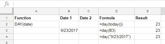
In cell E2, the formula returns the current day. As you can see, in cell E3, the formula returns the day from the given date in cell B3. Finally, the formula in cell E4 returns the day from a given date inside the formula.

NOW Function in Google Sheets

How to use the NOW function in Google Sheets?

The NOW Google Sheets function is similar to the TODAY function. The TODAY function returns only the current date. But the NOW function returns the DateTime. Needless to say, both are volatile.

=NOW()

Google Sheets MONTH Function

How to use the MONTH function in Google Sheets?

Syntax:

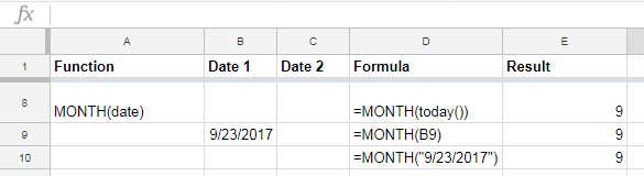
=MONTH(date)

Purpose: Google Sheets MONTH function returns the month (in numerical format) from a given date.

Arguments:

date – The particular date from which to extract the month.

Example of the MONTH function:

Google Sheets YEAR Function

How to use the YEAR function in Google Sheets?

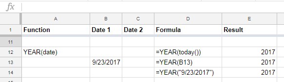
=YEAR(date)

Purpose: Google Sheets YEAR function returns the year (in numerical format) from a specific date.

Arguments:

date – It’s the date from which to extract the year.

See some example formulas for the YEAR function in Docs Sheets.

Standard Google Sheets Date Functions

As I have mentioned above, the above categorizations of Google Sheets Date functions are simply for explanation purposes. There is no such categorization in the real sense.

Let us begin with Standard Google Sheets Date functions.

Google Sheets DATE Function

How to use the DATE function in Google Sheets?

Syntax:

=DATE(year, month, day)

Purpose: Use the Google Sheets DATE function to convert a provided year, month, and day into a date.

Arguments:

year – It’s the year component of the date.

month – It’s the month component of the date.

day – It’s the day component of the date.

Example of the DATE function in Sheets.

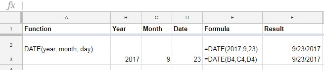
Sometimes we keep the year, month, and day in separate columns like in cells B3, C3, and D3 respectively. So this function is to return the date from such entry.

DATEVALUE Function in Google Sheets

How to use the Google Sheets DATEVALUE function?

Syntax:

=DATEVALUE(date_string)

This is one of the very useful date functions in Google Sheets.

Purpose: The Datevalue function converts a date stored as text to a serial number that Google Sheets recognizes as a date. You can later utilize the to_date() function to convert back that serial number to date.

Arguments:

date_string – It’s the string representing the date.

Usage Notes:

When you use a string inside the DATEVALUE formula you can apply different date formats. See the below example screenshot where I’ve applied different date formats inside the formula (except row # 10).

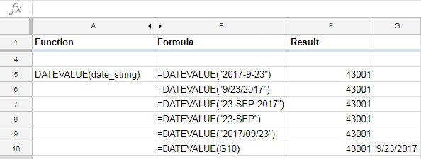
But when you use the DATEVALUE function to refer to a cell (refer to the formula in cell E10), that date should be entered as per the standard date format set on your spreadsheet.

You can check this by entering a date in any cell (cell G10 as per my example). If the entered value is a date, it would normally get aligned to the right.

Now format that date (in cell G10) to text from the menu Format > Number > Text. It won’t affect the DATEVALUE formula output.

Must Read: DATEVALUE Function in Google Sheets: Advanced Tips and Tricks.

DAYS Function in Google Doc Sheets

How to use the DAYS function in Google Sheets?

Syntax:

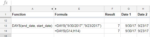
=DAYS(end_date, start_date)

Formula examples and purpose:

You can utilize this google sheets date function to find the date difference in number. That means the number of days between two given dates.

Normally the start date will be a past date and the end date will be a future date. If you use these dates on the reverse, the formula will return a negative number.

=DAYS("26/03/2019","26/04/2019")

Result: -34

Google Sheets DAYS360 Function

How to use the DAYS360 function in Google Sheets?

Syntax:

DAYS360(start_date, end_date, [method])

Purpose: Use to calculate the difference between two days based on the 360-day year.

Arguments:

start_date

end_date

method – Day count method indicator.

I have seen Google Sheets users wrongly using the DAYS360 function instead of the DAYS function. If you use DAYS360 without knowing the usage, you will get the wrong output.

Suppose if you just want to find the difference of days between two dates, use the function DAYS or DATEDIF.

Formula Example to the DAYS360 function in Sheets:

=DAYS360("30/03/2018", "31/03/2018", 1)

The above formula returns 0, not 1. Why?

Here at the end of the formula, I’ve used the day count indicator 1. It’s the European method where any start date or end date that falls on the 31st of a month (see the above dates in the formula), has its day of month changed to 30.

If you leave the method blank, the formula follows the US method in that if a start date is the last day of a month, the day of the month of the start date is changed to 30 for the purposes of the calculation.

In concise you can use the DAYS360 function in financial interest calculations.

Google Sheets Advanced Date Functions

Now let us see how to utilize some advanced date functions in Google Sheets. These functions are also simple but as a beginner, some of you may find a tough time with them. That is why I put it under advanced date functions. Here we go!

EDATE Function in Google Doc Sheets

How to use the EDATE function in Google Sheets?

A very useful date function in Google Sheets which will come in handy in date-related conditional formatting.

Syntax:

=EDATE(start_date, months)

Arguments:

start_date

months – The number of months before (-ve) or after (+ve) the ‘start_date’ to calculate.

Purpose:

Use Google Sheets EDATE date function to return a date after or before a given date based on the number of months as input.

For example, you can get a date after six months after a given date or 5 months back from a given date. That month’s part is important. See the formulas below.

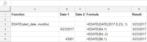
This function also accepts date value, see the DATEVALUE function, which is already detailed above.

Google Sheets ISOWEEKNUM Function

How to use the ISOWEEKNUM function in Google Sheets?

Syntax:

=ISOWEEKNUM(date)

To understand this Google Sheets function, you should first know what is ISO Week. This Wiki article will be helpful to you to know about ISO Week in detail.

ISO Week in a Nutshell:

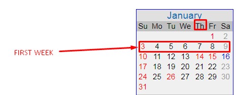
The ISOWEEKNUM function follows the ISO 8601 date and time standard.
In this standard weeks begin on Monday and end on Sunday.
As per this standard, Week 1 of the year is the week that contains the first Thursday of the year.

See the below image.

Formula examples of the ISOWEEKNUM function in Sheets:

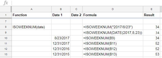
The above ISOWEEKNUM formulas return the numbers of the ISO weeks of the year where the provided date falls.

NETWORKDAYS Function in Google Doc Sheets

How to use the NETWORKDAYS function in Google Sheets?

Syntax:

=NETWORKDAYS(start_date, end_date, [holidays])

You can utilize the NETWORKDAYS function to get the number of networking days between two given dates. Then what are networking days?

Normally networking days are the total number of days excluding weekends. Weekends here means Saturday and Sunday. If you want to change the weekends there is another function, that follows after this.

Optionally you can exclude holidays also. Examples are always the best method to learn.

See how I have excluded the US Federal holidays in 2019 in the networking day count.

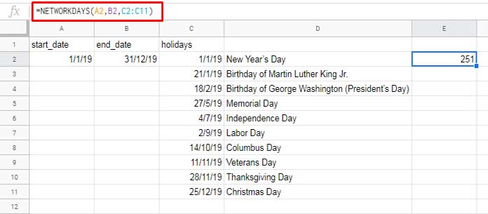
exclude holidays in network day calculation

If any of the provided holidays fall on weekends, it won’t get deducted twice.

To cut short this tutorial as well as to make things simple, I’ve opted out of the string method this time. The same will be followed in the coming examples.

Google Sheets NETWORKDAYS.INTL Function

This is one of my favorite Google Sheets Date functions. You will also agree to it once you learn it.

How to use the NETWORKDAYS.INTL function in Google Sheets?

Syntax:

=NETWORKDAYS.INTL(start_date, end_date, [weekend], [holidays])

This function is superior to NETWORKDAYS. How?

The NETWORKDAYS.INTL is almost the same as the NETWORKDAYS function. The only difference is, the former function allows you to specify the weekends.

This is useful when in some countries like the middle east, Friday and Saturday are considered weekends.

To use NETWORKDAYS.INTL function, you should know the weekend numbers.

What are the Weekend Numbers in Google Sheets?

If weekends are 2 days;

Saturday, Sunday – Weekend Number is 1.
Sunday, Monday – Weekend Number is 2.
Monday, Tuesday – Weekend Number is 3.
Tuesday, Wednesday – Weekend Number is 4.
Wednesday, Thursday – Weekend Number is 5.
Thursday, Friday – Weekend Number is 6.
Friday, Saturday – Weekend Number is 7.

If the weekend is 1 day only;

Sunday only – Weekend Number is 11.
Monday only – Weekend Number is 12.
Tuesday only – Weekend Number is 13.
Wednesday only – Weekend Number is 14.
Thursday only – Weekend Number is 15.
Friday only – Weekend Number is 16.
Saturday only – Weekend Number is 17.

Now let us go through two example formulas.

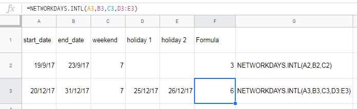
Example to NETWORKDAYS.INTL function in Google Sheets

To understand the above NETWORKDAYS.INTL formula in cell F3, see the below calendar.

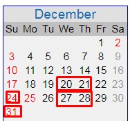
In the formula, what I want is to find the working days during the period from 20/12/2017 to 31/12/2017. The holidays are on 25/12/2017 and 26/12/2017.

I have used the weekend number 7 in the formula, which denotes weekends as Friday and Saturday.

So the remaining days I’ve marked in the above calendar and when you count it, you will get the number 6 and that is the result of the formula.

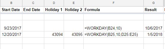
WORKDAY Function in Google Sheets

How to use the WORKDAY function in Google Sheets?

Syntax:

=WORKDAY(start_date, num_days, [holidays])

The WORKDAY function has lots of similarities with the NETWORKDAYS function which I have already detailed above.

We utilize NETWORKDAY to find the number of working days between two given dates excluding weekends and holidays.

Here in WORKDAY, we can find a date after a given number of working days.

Suppose today is 01/01/2017. We can use the WORKDAY function to find a date after 90 working days. Working days means days excluding weekends and holidays.

First please learn the above NETWORKDAYS function then come back to the WORKDAY function so that you can easily grasp it.

Helpful Tips: Use a negative number in place of num_days to count backward.

Google Sheets WORKDAY.INTL Function

How to use the WORKDAY.INTL function in Google Sheets?

Syntax:

=WORKDAY.INTL(start_date, num_days, [weekend], [holidays])

All the Google Sheets date functions ending with INTL are so special to me. Such Google Sheets date functions will be useful if you have employees deployed around the world. Because weekends, as well as holidays, may differ among countries.

The WORKDAY.INTL function is the same as the WORKDAY function. But here the difference is, you can change the weekend days.

Please refer to NETWORKDAY.INTL function and then the WORKDAY function above. Then come back here.

You can use WORKDAY.INTL function to return date after giving input as the number of working days.

Suppose today is 01/01/2017. You want to find a future date after 180 working days. Additionally, you want to exclude the weekends of your choice and your selected holidays. Then use WORKDAY.INTL function.

There are weekend codes or identification numbers that are required in the function. Find it above under the function NETWORKDAYS.INTL.

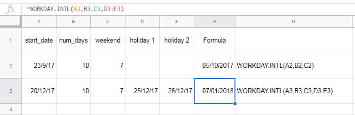
Formula example to the WORKDAY.INTL function Sheets

Here in this example, I’ve used weekend number 7 which indicates Friday and Saturday as weekends. If you want to use Saturday and Sunday as weekend days, use weekend number 1.

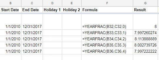
YEARFRAC Function in Google Sheets

How to use the YEARFRAC function in Google Sheets?

Syntax:

=YEARFRAC(start_date, end_date, [day_count_convention])

YEARFRAC is yet another useful Google Sheets date function. Use this date function to return the number of years including fractional years between two given dates.

In the YEARFRAC formula, you can specify which day count conversion to be followed. There are four different day count conversions in Google Sheets.

What is the day count conversion?

It is like how many days in a year to be considered. Whether it’s 360 days as a year or 365 days or the actual number of days in a year as the year.

Day counts conversion numbers.

0 indicates 30 days each month. That means 360 days in a year, i.e. 30/360.
1 indicates actual days between two specified days, i.e. actual/actual.
2 indicates the actual number of days between two specified days but assumes a 360-day year, i.e. actual/360.
3 indicates the actual number of days between two specified days but assumes a 365-day year i.e. actual/365.
4 is similar to 0, this calculates based on a 30-day month and 360-day year but adjusts end-of-month dates according to European financial conventions, i.e. European 30/360.

Confused? Don’t worry! I have included all the above count conversion numbers within the below formulas. Also, detailed information about the count conversion numbers can be found on this Wiki page.

Formula examples of the YEARFRAC function in Google Sheets.

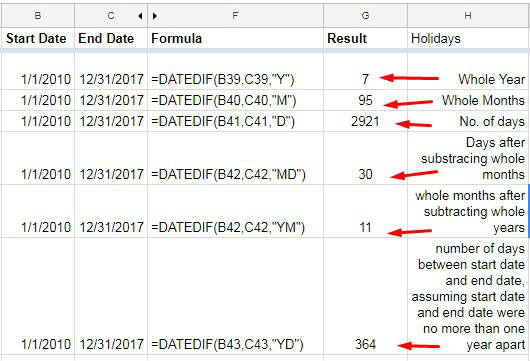
DATEDIF Function in Google Sheets

How to use the DATEDIF function in Google Sheets?

Syntax:

=DATEDIF(start_date, end_date, unit)

DATEDIF is one of the very useful functions among the available Google Sheets Date Functions. This is not a DATED IF function. It is a DATE DIF function. What’s it?

This function will do the job of three functions. What are they? The DATEDIF function calculates the number of days, months, or years between two given dates with the help of a unit abbreviation.

What is the “unit” in the syntax?

It’s a text abbreviation for the unit of time. Where;

“Y” stands for the number of whole years between a start date and an end date.
“M” stands for the number of whole months between a start date and an end date.
“D” stands for the number of days between a start date and an end date.
“MD” stands for the number of days between a start date and end date but after subtracting whole months.
‘YM” stands for the number of whole months after subtracting whole years.
“YD” stands for the number of days between a start date and an end date, assuming the start date and end date were no more than one year apart.

Example of the DATEDIF function in Docs Sheets:

Google Sheets WEEKDAY Function

How to use the WEEKDAY function in Google Sheets?

Syntax:

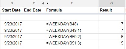
=WEEKDAY(date, type)

Purpose: The WEEKDAY function in Sheets returns a number representing the day of the week of the provided date.

First I will tell you what is the “type” in the WEEKDAY date function.

Type is optional in the function. If omitted or put as 1, the day count will start from Sunday to Monday. In this case, the weekday number for Sunday would be 1 (Sunday 1, Monday 2, Tuesday 3, … Saturday 7).

If you put 2 then the counting will start from Monday to Sunday (Monday 1, Tuesday 2, Wednesday 3 … Sunday 7). See a few examples.

If you put 3 then the counting will start from Tuesday (1) to Monday (0), i.e., 1, 2, 3, 4, 5, 6, and 0 (not 7).

Google Sheets WEEKNUM Function

How to use the WEEKNUM function in Google Sheets?

Syntax:

=WEEKNUM(date, [type]

The WEEKNUM function returns a number representing the week of the year where the given date falls.

Similar to the WEEKDAY function you can determine which day to consider as the week start day.

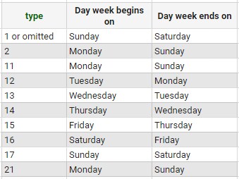
Note: The week containing January 1 will be numbered as week 1. This is applicable to types 1 to 17. In type 21, the week containing the first Thursday of the year is numbered as week 1.

Formula example to the WEEKNUM function in Sheets:

The formula in cell C2 which is dragged/copied down:

=weeknum(A2,2)

The formula in cell E2 which is also dragged/copied down:

=weeknum(A2,21)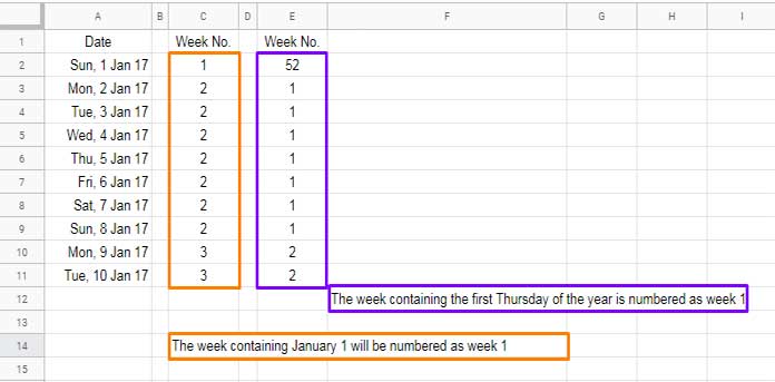

In both the formula types (type 2 and 21), the day week begins on Monday and the day week ends on Sunday.

Let us conclude this ultimate Google Sheets Date Functions tutorial. Now to the last function.

EOMONTH in Google Sheets

Syntax:

=EOMONTH(start_date, months)

This function simply returns the end of the month of a given date.

Suppose our date to be checked in cell C4 is 01/24/2017.

You can apply the formula below.

=eomonth(C4,0)

In this formula, “0” represents the current month. It will return the last date of the month, i.e., 01/31/2017.

If you change the value to “1”, it will return the next month’s last date and so on. Enter the below formula on your Sheet and check the output.

=eomonth(today(),-1)

Here is a more detailed tutorial: EOMONTH Function in Google Sheets: All About.

Conclusion

I don’t want to drag this tutorial anymore! Because I know already this tutorial got a bit lengthy.

I myself never thought this much time I would take to complete this tutorial. I took more than 10 hours at a stretch to complete this Google Sheets Date Functions tutorial! If you find it useful please share.

72 COMMENTS

Erin December 23, 2023 At 1:53 am

Hello! I loved this and have saved it for future use. Unfortunately, what I was originally looking for isn’t on it, and I am hoping you might be able to help.

I have two sheets. One sheet has pay dates, and the second sheet is bills with their due dates. I want to auto-highlight the bills on sheet 2 that fall between one payday and the next from sheet 1. I know I can use a formula and manually add the two dates, but I’d like to have the formula refer to the actual cell since the dates will change every month.

I know it will be a custom formula, but I’m stuck on how to refer to a cell on the other sheet.

In my head, it goes like this:

If column F on sheet 2 is before cell A2 on sheet 1, then highlight the entire row on sheet 2.

Thank you!!!

- Prashanth KV December 23, 2023 At 9:59 am
  
  To refer to another sheet, you need to use INDIRECT in conditional formatting.
  
  Here is the rule that you can try, assuming the sheet names are Sheet1 and Sheet2:
  
  =AND(ISDATE($F1), LT($F1, INDIRECT("Sheet1!A2")))
  
Sydney B July 6, 2023 At 3:42 am

How can I pull the date from the month, year, and weekday? Think of a calendar view. I need to build a formula that pulls the month (January), year (2023), and weekday (Monday) to pull the date (January 2). I imagine that I need to include the week number somewhere, which is fine. I appreciate your help!

- Prashanth July 7, 2023 At 12:55 pm
  
  Assume that cells B2, B3, and B4 contain the month text, year, and weekday text, respectively.
  
  For example:
  
  Cell B2 contains the text “February”.
  Cell B3 contains the number 2023.
  Cell B4 contains the text “Monday”.
  
  Then you can try the following formula:
  
  =LET(mon,LET(dt,DATE(B3,MONTH(B2&1),1),dt-WEEKDAY(dt,2)+ MATCH(B4,{"Monday","Tuesday","Wednesday","Thursday","Friday","Saturday","Sunday"},0)), IF(MONTH(mon)=MONTH(B2&1),mon,mon+7))
  
KenW February 1, 2023 At 2:50 am

I have a data set in a Google Sheet that captures employee time off requests for vacation, sick days, etc.

The data includes a Start Date column and an End Date column.

For example, someone is requesting vacation from 1/1/2023 to 1/15/2023.

I am trying to identify dupes (i.e., overlapping dates).

For example, if that same person enters another record later on for vacation from 1/10/2023 to 1/15/2023, we know that is impossible – they can’t be off “twice” on the same days.

What is the best way to capture those types of duplicates?

It’s not just the values on the columns, but the data range in between.

Thanks,
Ken

- Prashanth February 2, 2023 At 1:25 pm
  
  Hi, KenW,
  
  We can expand those dates using one of the new Lambda helper functions and find such duplicates.
  
  I have such a tutorial in the pipeline. If you share a sample of your Sheet, I may consider writing my formula/tutorial around that problem.
  
Elizabeth Hatch December 29, 2022 At 12:25 am

Hi!

I would like to create a header in my spreadsheet with the days of the month in increments of two days from 1-29, starting with the TODAY function; for 3 months.

I can do it for the first month by setting TODAY in the first cell and then adding two to the next cell over, copying it into the rest of the row up to 29.

Is there a function I can use to refer back to the first cell and start this sequence again in the next month (1-29), and then again in the third month?

Thanks for any help you can give.

- Prashanth December 29, 2022 At 5:25 pm
  
  Hi, Elizabeth Hatch,
  
  Give this array formula a try.
  
  Assume the first date is in cell A1.
  
  =lambda(final,filter(final,final<>""))({ifna(lambda(data, filter(data,data<=date(year(A1),month(A1),min(29,day(eomonth(A1,0)))))) (sequence(1,16,A1+2,2))),lambda(data,filter(data, data<=date(year(eomonth(A1,0)+1),month(eomonth(A1,0)+1), min(29,day(eomonth(eomonth(A1,0)+1,0))))))(sequence(1,16,eomonth(A1,0)+1,2)),lambda(data, filter(data,data<=date(year(eomonth(A1,1)+1), month(eomonth(A1,1)+1),min(29,day(eomonth(eomonth(A1,1)+1,0)))))) (sequence(1,16,eomonth(A1,1)+1,2))})
  
  It requires a blank row to populate the dates.
  
  - Prashanth December 29, 2022 At 6:23 pm
    
    The result must be formatted to Format > Number > Date.
    
Michelle L Adams November 3, 2022 At 2:07 pm

Hello! I would like to enter a date of a document that needs to be redone every 6 months.

At 5 months, I would like it to highlight yellow, and at the 6-month point, I would like it to be highlighted red.

Can I do this?

- Prashanth November 4, 2022 At 12:02 pm
  
  Hi, Michelle L Adams,
  
  Try these formulas.
  
  Yellow – =isbetween($F3,edate(today(),-6),edate(today(),-5),false)
  
  Red – =and(isdate($F3),lte($F3,edate(today(),-6)))
  
Zman September 20, 2022 At 10:40 am

Hi there,

I wonder if you can help me with my dilemma.

I have a list of dates and values.

I want to calculate the average values in a range for the last 7 “workdays” – a 7-day running average.

I can do it with the calculation of today -7 days, but I can’t get it to work with workday(cell ref, -7 workdays).

- Prashanth September 23, 2022 At 8:27 am
  
  Hi, Zman,
  
  Assume the criteria range (date) is column C (C1:C) and the average range is column B (B1:B).
  
  Then try this formula which uses the newly introduced MAP function.
  
  =AVERAGEIF(map(C1:C,lambda(wd,iferror(and(workday(wd-1,1)=wd,isbetween(wd,WORKDAY(today(),-7),today()))))),TRUE,B1:B)
  
B4ALLB4U August 8, 2022 At 1:07 pm

Hello, Thanks for your hard work.

I want to restrict users to select the date only three days from the current date.

If the user entered date is more than three days, the system has to show a pop-up error message and not accept the date in the column.

If the date is below three days, the system has to accept the date in the column.

Please guide me on how to set the above condition in Google sheets.

- Prashanth August 9, 2022 At 4:46 pm
  
  Hi, B4ALLB4U,
  
  You can do it as follows.
  
  Select the cells and go to Data > Data validation > Criteria > Date > On or before.
  
  Enter the following formula in the given field.
  
  =today()+3
  
  Check “Reject Input” and “Save.”
  
YAGNESH DARJI April 24, 2022 At 2:52 pm

Thank you very much for this Effort.

I want to find the “LOW” Price of a particular stock for a given month.

Tried your “high” formulae in the same manner for getting low but were unable.

=index(sortn(GoogleFinance($A$1,"high",B118, C118,"DAILY"),2,1,2,0),2,2)

$A$1 = STOCK SYMBOL
B118 = 3/2/2022
C118 = 3/31/2022

- Prashanth April 25, 2022 At 9:16 am
  
  Hi, Yagnesh Darji,
  
  I assume you were trying to find the MIN of the above historical data, not the low price for the specified date(s).
  
  If so, try this.
  
  =index(sortn(GoogleFinance($A$1,"high",B118, C118,"DAILY"),1,1,2,1),0,2)
  
Koleen April 21, 2022 At 9:14 pm

Thank you for this tutorial! I may have missed where I can auto-populate due dates from the event date. For example,

The event date is April 25, 2022, and is located in cell D1.

I have 25 tasks to complete before April 25 – these tasks are due in various increments – 30 days out; 25 days out; 5 days out… etc. and are listed in D4 through D21. Some will be + for tasks after the event.

I need to auto-populate those due dates. What would my formula be?

Thank you!

- Prashanth April 23, 2022 At 9:56 am
  
  Hi, Koleen,
  
  It requires a sample sheet for me to answer. Please feel free to share one in the comment reply below.
  
GJ April 16, 2022 At 5:13 pm

Hi. Thank you for this. How would I formulate the start of a pay period and the end of a pay period given the pay date?

Let’s say the pay date is Friday, Jan 14th, 2022.

I want my sheet to auto-populate the pay period start date (Saturday, Jan 1st, 2022) and the pay period end date (Friday, Jan 7th, 2022) by itself.

I want my sheet to recognize the start date as Saturday and the end date as Friday.

- Prashanth April 17, 2022 At 3:32 pm
  
  Hi, GJ,
  
  Let’s assume the pay date is in D4.
  
  To get the payment period, use the below formulas.
  
  Start: =(D4-weekday(D4)+6)-13
  
  End: =(D4-weekday(D4)+6)-7
  
  If the above doesn’t help, please share a few more examples in your reply.
  
Sam Stern April 1, 2022 At 6:29 pm

You’re a wizard. Here’s my problem. I would be so appreciative.

Looking to add to dates (e.g., =A1+7), but if the end date is a weekend or holiday, push it to the next workday.

My difficulty is that WORKDAY and adding holidays to it will not count them *within* the seven days, but I want to include them, but not if it’s the 7th day itself.

Assume I can array holidays and if needed, weekends.

Thank you in advance!

- Prashanth April 3, 2022 At 2:48 pm
  
  Hi, Sam Stern,
  
  Just enter the holidays (not weekends) in B1:B.
  
  Then try the below formula in C1.
  
  =workday(A1+7-1,1,B1:B)
  
Lexi Maitland January 27, 2022 At 6:49 am

Hi! This was so helpful.

I’m looking to measure Projected Date vs. Actual Date.

B1 (Projected Date) = 1/26/22
C1 (Actual Date) = 1/27/22

The percentage is 100% if the dates are the same.

If the dates are not the same, return the percentage.

Thank you for your time and assistance!!

- Prashanth January 28, 2022 At 11:44 am
  
  Hi, Lexi Maitland,
  
  This may possible if you have a start date.
  
  E.g.:
  A2 (Start Date)
  B2 (Projected Completion Date) = 1/26/22
  C2 (Actual Completion Date) = 1/27/22
  D2 (Duration in Percentage)
  
  =to_percent(days(C2,A2)/days(B2,A2))
  
  It will return 100% if the dates are the same.
  
George January 5, 2022 At 3:26 pm

Hello, I am trying to make a formula that allows me to select a date from the sheets’ calendar but can’t do it. (I want to be able to click on a shell and then get a calendar to select the date)

Thank you in advance, and have a great 2022!

- Prashanth January 6, 2022 At 12:49 pm
  
  Hi, George,
  
  Please follow this – How to Get Date Picker in Blank Cell in Google Sheets.
  
  Thanks.
  
Proserpine December 3, 2021 At 10:37 am

Hi, I love this tutorial. I was able to use some of the functions.

I just have questions on how I can compute if on cell A1 I have a specific date, and on cell B1, I have 6 (represents six months).

How can I have A1 +B1 = C1?

Like A1 (1-19-2021) + B1 (6 months) = C1 (7-19-2021)

I hope you can help me. Thank you.

- Prashanth December 3, 2021 At 10:52 am
  
  Hi, Proserpine,
  
  You can use the EDATE function as below in cell C1.
  
  =edate(A1,B1)
  
  Assume A1 has a valid date and B1 has the number 6.
  
Nitin Jain September 20, 2021 At 11:26 pm

Hi Prashanth,

Thank you for helping out with Google Sheets.

Can you please assist me in Validating the same case for the Google Form?

- Prashanth September 21, 2021 At 9:02 am
  
  Hi, Nitin Jain,
  
  At present, Google Form doesn’t support it. There might be add-ons available for the same.
  
Nitin Jain September 19, 2021 At 12:14 am

Hi,

I am looking for a formula to validate whether the given DOB falls in 18 years to 45 years or not?

It should be through validation, and if he doesn’t fall in the 18 to 45 years range, show validation help text “You are not eligible.”

Thanks

- Prashanth September 19, 2021 At 7:07 am
  
  Hi, Nitin Jain,
  
  Assume the cell in question is B2.
  
  Go to DATA > Data Validation. Choose the Criteria “Custom formula is” and enter the below rule in the given field there.
  
  =and( isdate(B2), gte(datedif(B2,today(),"Y"),18), lte(datedif(B2,today(),"Y"),45) )
  
  You can learn the use of the GTE and LTE functions here – Comparison Operators in Google Sheets and Equivalent Functions.
  
  Note:- To apply the rule to a range like B2:B100, just change the “Cell range” accordingly within the Data Validation dialogue box. The formula will be the same.
  
Brian M July 8, 2021 At 10:47 pm

Hello,

The tutorial was great. I used a few formulas already.

I am trying to find a way to calculate how many projects are past their renewal dates. So I have column A with dates, and I want to calculate how many projects are past today’s date, automatically without changing the date each time. Is there a way to calculate a total?

- Prashanth July 9, 2021 At 9:18 am
  
  Hi, Brian M,
  
  Use the Countif() with today() as below.
  
  =countif(A1:A,"<"&today())
  
Steven Umpleby June 17, 2021 At 1:58 pm

Hi Prashanth,

You helped me out with the formula below. Is it possible to select two weeks from a selected date?

=ArrayFormula(sumifs(D5:D,B5:B,B2,month(C5:C),C2))

Cheers
Steve

- Prashanth June 17, 2021 At 4:17 pm
  
  Hi, Steven Umpleby,
  
  You can try this formula.
  
  =ArrayFormula(sumifs(D5:D,B5:B,B2,C5:C,">="&C2,C5:C,"<="&C2+14))
  
  Note:- Please replace the earlier formula (month number) with the below one.
  
  =ArrayFormula(sumifs(D5:D,B5:B,B2,datevalue(C5:C),">0",month(C5:C),C2))
  
Andrew Dahler March 19, 2021 At 11:23 pm

Trying to calculate how many days it takes us to complete our job process.

We currently add a new job every day.

I am using NETWORKDAYS – Column A contains our start date and Column B contains our finish date.

This works great as long as there is a date entered into the “finish date” field.

If we have not completed this task, it shows up as a -31580.

These jobs are not completed in numerical order.

Is there a way to have the NETWORKDAYS formula ignore blank fields in the hopes of alleviating the negative numbers as well as the need to update the formula in that field, every time a process is completed?

Any help?

- Prashanth March 21, 2021 At 12:08 pm
  
  Hi, Andrew Dahler,
  
  This formula may help?
  
  =if(iferror(datevalue(A2)*datevalue(B2))>0,networkdays(A2,B2),0)
  
  The formula would output 0 in such cases. If you want blank, just remove the 0 that you can find in the last part of the formula.
  
- Prashanth March 28, 2021 At 4:03 pm
  
  Hi, Andrew Dahler,
  
  If you want examples, please follow this tutorial.
  
  Calculate Number of Days Ignoring Blank Cells In Google Sheets – Array and Non-Array Formulas
  
kris hart January 29, 2021 At 1:19 am

Hoping you can help me.

I’ve read through your entire article and my head is spinning.

We own a storage yard for containers to be stored. We have to charge customers from the day they begin to store a container here to the day it leaves our yard.

When I enter the start date and the end date and use the =DAYS or =DATEDIF, OR =MINUS(A2,B2) the result is not including the day they begin.

For example, 1/1/2021 – 1/7/2021 is calculating 6 days when we would bill 7 days.

- Prashanth January 29, 2021 At 10:05 am
  
  Hi, kris hart,
  
  The date difference between 01/01/2021 and 01/01/2021 will be 0.
  
  So, if A1 contains 01/01/2021 and B1 contains 02/01/2021 (both in DD/MM/YYYY format as per my sheets’ formatting), the following formula will return 1.
  
  =days(B1,A1)
  
  To make both the dates inclusive, modify the formula as below.
  
  =days(B1,A1)+1
  
Carmen January 26, 2021 At 11:21 pm

Hi, I need help with Google Sheets formatting of dates.

If I have two columns:
Column E – to be filled with dates
Column F – 90 days from date in Column E

How can I get Column F to be filled in automatically when I key in dates in Column E?

- Prashanth January 27, 2021 At 4:02 pm
  
  Hi, Carmen,
  
  If you start entering the dates from E2 (in E2:E as cell E1 may contain a label), then you can try the below array formula.
  
  =ArrayFormula(TO_DATE(IFERROR(if(DATEVALUE(E2:E),E2:E+90,))))
  
  Empty column F and insert the formula in cell F2.
  
Paul wurz December 25, 2020 At 12:21 am

Hi, Can you help me find a formula for my Google Sheets?

Example:
A1: 160000
A2: 15000
A3: =(date)
A4: =sum(A1-A2) starting from cell A3

I need to subtract cell A2 from cell A1 every 30 days into cell A4.

- Prashanth December 25, 2020 At 10:28 am
  
  Hi, Paul wurz,
  
  This may require an Apps Script which I’m not familiar with.
  
  Please try asking the corresponding community here – https://developers.google.com/apps-script/community
  
Rps December 22, 2020 At 12:57 am

The week from Friday to Thursday, what is formula last week and update automatically.

- Prashanth December 22, 2020 At 11:14 am
  
  Hi, Rps,
  
  Dates in A2:A.
  
  To filter the last week’s dates (Friday-Thursday) from this date range, use the below formula.
  
  =filter(A2:A,weeknum(A2:A,15)=weeknum(today(),15)-1)
  
Kayi December 12, 2020 At 3:55 am

Hi,

I have a column from Google Sheets with a date on it. Column B.

I need Column A to calculate the date to show the Monday of that week.

I have this formula that works, B2-WEEKDAY(B2,3), but I need to make it an array so it auto-fills. How can I do this?

- Prashanth December 12, 2020 At 8:31 am
  
  Hi, Kayi,
  
  Formula:
  
  =ArrayFormula(to_date(if(len(B2:B),B2:B-WEEKDAY(B2:B,3),)))
  
  Make column A empty, then insert this formula in A2.
  
Hardest Easy November 18, 2020 At 8:19 am

Hello,

I am trying to display the $ value present in a cell associated with the last day of each month given a daily $ value is collected in a spreadsheet each day. How can you only collect that last day of each month (12 values) among 365 values in a year?

- Prashanth November 19, 2020 At 8:25 am
  
  Hi, Hardest Easy,
  
  Assume the said two columns are A2:A (dates) and B2:B (dollar values). The cells A1 and B1 contain the labels.
  
  If so, try this formula.
  
  =array_constrain(sort(sortn(sort({A2:B,month(A2:A)},1,0),9^9,2,3,0)),9^9,2)
  
  The formula must be adjusted as per your LOCALE settings as detailed here – How to Change a Non-Regional Google Sheets Formula.
  
  If you want the formula explanation, please mention that in your reply.
  
Bijon SARKAR June 13, 2020 At 8:05 am

I’ll try to explain my problem, please help.

Id of Crew|Name|In|Out|D.Hrs|Night D.Hrs
N10001|AAA|05-06-2020 16:00|05-06-2020 23:00|07:00|01:00 (btn 22 to 06)
N10002|BBB|06-06-2020 23:00|07-06-2020 08:00|09:00|08:00 (btn 22 to 06)
N10006|XYX|08-06-2020 03:00|09-06-2020 23:30|20:30|03:00 (btn 22 to 06)
N10010|LMN|08-06-2020 21:00|08-06-2020 23:45|02:45|01:45 (btn 22 to 06)

- G T August 26, 2020 At 2:20 pm
  
  Hi Bijon,
  
  I think your formula will be this.
  
  Hours = 24 * (Out – In)
  
  You don’t even need a formula.
  
  Geoff
  
Tracy DeCrosta June 12, 2020 At 2:22 am

I would like to turn a cell red if it is five years from the date listed in the cell. Is this possible with google sheets?

- Prashanth June 12, 2020 At 10:29 am
  
  Can you explain a little more, please?
  
  The date in which cell and which cell do you want to turn to read on which date.
  
Bijon SARKAR June 11, 2020 At 10:41 pm

Hello,

Could anybody help me?

I want calculating night duty Hrs between two date-time. i.e.,

One who joining his duty at dd/mm/yyyy 10:00:00 hrs and out from duty at dd/mm/yyyy 04:45:00 hrs.

I want to calculate how many Hrs having worked between 22:00 to 06:00 between joining and outing his duty. (excel sheet or Google Sheet only).

Jon January 27, 2020 At 6:22 am

I’m trying to keep up with my monthly dues, and on my Google Sheet, I want the whole row to be highlighted if the due date is today.

I know how to highlight the whole row, but I don’t know how to automatically change the date on the cell.

For example, I would initially enter January 26 in the cell. After January 26, I want it to change to February 26 so that in conditional formatting, I can highlight any row with today’s date (every 26th).

- Prashanth January 27, 2020 At 9:36 am
  
  Hi, Jon,
  
  To know how to advance dates you can check this guide.
  
  Get a Dynamic Date that Advances/Resets in Google Sheets
  
  But I think the following formula will work in your case.
  
  If the said date is in cell B5, to highlight entire row # 5 on every 26th, select row # 5, and use this =day(today())=26 formula in conditional formatting.
  
Terry Heath September 12, 2019 At 6:07 pm

Worked it out…

=sumproduct(text(Data!A:A, "mm/yyyy")=text(today(), "mm/yyyy"), Data!E:E)

This works!

Terry Heath September 12, 2019 At 3:01 pm

Hello,

Could you help me?

I have a dashboard that shows the running totals of sales for the day, week and month.

I have managed to program formula for day & week but I am struggling with calculating sales in the current month.

My data is set out with a transaction date in column A and transaction total in column I.

This set of data is continually updated through an automated workflow integration.

To calculate weekly total I use this formula: sum(filter(Zapier!I:I,weeknum(Zapier!A:A,2)=weeknum(today(),2)))

Is there a formula that would do the same for a monthly total?

Thank you in advance for your assistance

Erin August 28, 2019 At 7:03 pm

Hi Prashanth,

I thought your response to Anakowi on June 16, 2019, might provide the answer for which I’ve been searching!

Unfortunately, though, when I plugged it into my Google Sheets document, it did not work as I’d hoped. I’ll explain what I need and hopefully, you can advise me accordingly! Thanks, so much, in advance!!

So, I’ve created a file to include all of the coupons and sales ads, including item type, brand, store, sale amount, and each coupon’s date of expiration.

What I want to have happened is… whenever the expiration date is TODAY, the cell is (let’s say) RED. When it is within the next 7 days, I want the cell to be GREEN. If the expiration date is 7-14 days from today, I want it to be YELLOW.

I’ve now tried your suggestion to the most recent poster, as well as another blogger’s suggestion, which is as follows:

Format Rules –> Format Cells if — >
Custom Formula IS –>

=if(WEEKNUM((INDIRECT("B"&ROW())))=WEEKNUM((TODAY()+7), 1), 1,0)=1

Formatting Style –>

YELLOW (Fill Bucket color selection)

However, neither option has worked… am I missing something or what do you suggest?

Thanks in advance!

- Prashanth August 29, 2019 At 9:55 am
  Hi, Erin,
  
  I have a similar tutorial here – How to Highlight Cells Based on Expiry Date in Google Sheets.
  I have my expiry dates in B2:B. Here are the conditions and custom formulas to highlight B2:B based on expiry.
  
  Condition 1: Highlight the cell to Red, if the expiration date is Today.
  Formula Rule 1: =B2=today()
  Note: If you want to highlight multiple columns, I mean B2:Z instead of B2:B, use it as =$B2=today().
  
  See this guide for detailed info – Highlight an Entire Row in Conditional Formatting in Google Sheets.
  
  Condition 2: Expiry date is within the next 7 days, I want the cell to be in Green.
  Formula Rule 2: =and(B2>today(),B2<=today()+7)
  
  Condition 3: If the expiration date is 7-14 days from today, I want to highlight the cell to Yellow.
  Formula Rule 3: =and(B2>today()+7,B2<=today()+14)
Anakowi June 15, 2019 At 7:59 pm

Thank you, Prashanth. This info has been so useful.

I’m now stuck trying to automate the display of a date based on TODAY’s date to use with other calculations. I want the display date to always be “Friday” (start_date) and only changes when the next Friday is reached.

For example, today is Sat, 15 June 2019. So the display date will be Fri, 14 June 2019 until the next Friday arrives, i.e., Fri, 21 June 2019. Is it possible?

I’ve tried using WEEKNUM as the closest method to set Friday as the first day of the week, but it’s not giving me the result I need.

- Prashanth June 16, 2019 At 9:48 am
  
  Hi, Anakowi,
  
  That’s possible and detailed here – Get a Dynamic Date that Advances/Resets in Google Sheets.
  
  Here is the formula for your case.
  
  =TODAY()-MOD(TODAY()-date(2019,6,14),7)
  
  You can replace date(2019,6,14) with any cell reference. Further, the output may be in DATEVALUE. If so, you may need to format the output cell to date from Format > Number > Date.
  
  Best,
  
  Prashanth KV
  
Danny Alva January 24, 2019 At 2:00 am

I’m trying to set my utility bills schedule and the dates to show the upcoming payment date. So If the BILLING DATE is past the CURRENT DATE it should change the MONTH to the next.

Any help would be appreciated,

- Prashanth January 24, 2019 At 8:06 am
  
  Hi, Danny Alva,
  
  Assume your billing date, upcoming payment date, is in cell B1. If so, in cell C1, you can try this formula.
  
  Cheers!
  
- Prashanth February 10, 2019 At 9:15 am
  
  Hi, Danny Alva.
  
  I have just found that the formula was missing in my earlier reply due to some technical issue. So I have pasted the formula as an image this time. Please check.
  
  Thanks.
  
Vijay November 17, 2018 At 2:24 am

Thanks for your extremely useful article. Could I get your help in getting a couple of dates as below?

1. The date of the Friday last week

2. The date of the Friday Last month.

Much Appreciated.

Vijay

- Prashanth November 17, 2018 At 8:50 am
  
  Hi, Vijay,
  
  To find the date of the last Friday, you can try;
  
  =TODAY()-WEEKDAY(TODAY())-1
  
  This is based on the Weekstart Date and End Date calculation.
  
  But I am unsure about your second question.
  
  You may try this.
  
  =edate(today(),-1)-WEEKDAY(edate(today(),-1))-1
  
Seth June 20, 2018 At 12:53 am

Hi, thanks for this. Very useful. Any clue how to enter a function that will always display the date of a particular upcoming day? For example, I want a cell to display the date of next Tuesday up to and including that Tuesday. On the Wednesday after that Tuesday I want it to display the following Tuesday’s date.

- Prashanth June 20, 2018 At 9:42 am
  
  Hi, Seth,
  
  Welcome to InfoInspired!
  
  You can try the below formula. Replace the cell reference G1 with weekday numbers. 1 represents Sunday, 2 for Monday and so on. If you put 1 in G1 or replace G1 with 1, the formula would populate the dates from today to coming Sunday.
  
  =ArrayFormula(if(weekday(today())>G1,row(indirect("A"&TODAY()&":"&today()-weekday(today())+7+G1)),row(indirect("A"&TODAY()&":"&today()-weekday(today())+G1))))
  
  Cheers!