The CHAR function in Google Sheets converts a given number into a character based on the current Unicode table. It allows us to insert characters that are not readily available on the keyboard into the sheet.

I frequently use the Google Sheets CHAR function to insert a newline character in formulas and to include superscript/subscript characters.

To insert a new line (line break) within a cell, you can use the keyboard shortcut Alt + Enter on Windows or Option + Return on Mac. In formula results, you can achieve the same effect by using the relevant CHAR formula.

Another common use of this function is to create a 5-star rating system. However, with the introduction of the new rating smart chip, CHAR is no longer necessary for this purpose.

Additionally, CHAR can be employed in FILTER or QUERY functions to filter a table by matching characters in a column. Explore these tips and tricks in this tutorial.

How to Use Google Sheets CHAR Function

We can use the CHAR function to convert a number into an associated character. Which number, you might ask? We’ll get to that shortly. But first, let’s take a look at the syntax of the CHAR function in Google Sheets:

Syntax:

CHAR(table_number)

In this syntax, table_number represents the number you want to convert into a character.

The table_number can be any valid decimal number, which you can locate in this Unicode table. This table encompasses the complete set of basic UNICODE numbers.

Formula Examples

In the example below (screenshot), you can observe some of the table_numbers in column A, the characters these numbers represent in column B and the formulas in column C.

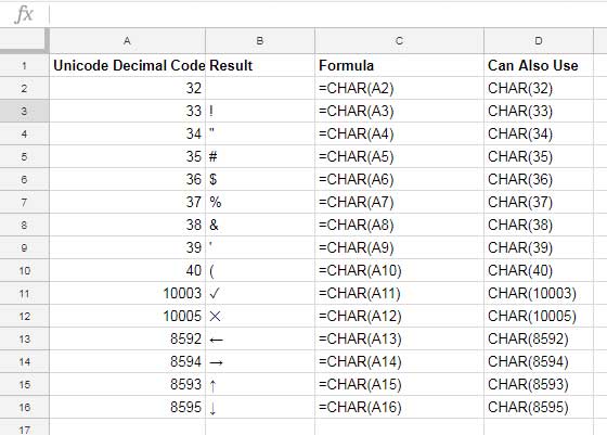
In summary, to obtain the check mark, you can use =CHAR(10003), and to get the cross mark, you can use =CHAR(10005).

I usually employ a SEQUENCE formula in cell A1 of a blank sheet to generate numbers from 1 to 12000 and an Array formula in cell B1 to generate the corresponding characters. You can then scroll down to locate the desired characters. Here are the two formulas:

=SEQUENCE(12000)
=ArrayFormula(CHAR(A:A))

CHAR is a non-array function in Google Sheets. Therefore, when you intend to use it in an array, you should utilize the ArrayFormula function to extend its functionality.

Here are some of my favorite useful characters:

1. =CHAR(169): © Copyright symbol
2. =CHAR(174) : ® Registered trademark symbol
3. =CHAR(181) : µ Micro sign
4. =CHAR(8593) : ↑ Up arrow
5. =CHAR(8595) : ↓ Down arrow
6. =CHAR(9200) : ⏰ Clock
7. =CHAR(9203) :⏳ Hourglass
8. =CHAR(9940): ⛔ No entry
9. =CHAR(9989): ✅ Check mark button
10. =CHAR(10062): ❎ Cross mark button

Advanced Use of CHAR Function in Google Sheets

I’ve already written a few tutorials that use the CHAR function in Google Sheets. The star rating mentioned at the very beginning is one of them.

Another application is adding superscript and subscript characters. This is particularly useful when you want to include molecular formulas in your spreadsheet. Here is the relevant tutorial: Google Sheets: Add Subscript and Superscript Numbers.

Here are a few more tutorials:

1. Inserting Bullet Points in Google Sheets.
2. Insert Special Characters Without Add-on in Google Sheets.
3. Smileys and Icons Based on Values in Google Sheets.
4. Start New Lines Within a Cell in Google Sheets – Desktop and Mobile.

Using CHAR Formula as a Delimiter in JOIN or TEXTJOIN

We typically combine keywords, first and last names, etc., using “&” or functions like JOIN, TEXTJOIN, and others.

Most often, we use JOIN or TEXTJOIN to join texts and insert a delimiter that separates the joined text. Common delimiters include “,”, or “|”.

However, if these delimiters are part of the joined text, they may cause issues later when you want to split the joined text using the same delimiter.

To avoid these issues, you can use the CHAR function in the delimiter part. Here’s an example:

Suppose you have the text “Apple, Orange” in cell C1 and “Carrot, Asparagus, Tomato” in cell D1. The following formula will return the text “Apple, Orange❄Carrot, Asparagus, Tomato.”

=JOIN(CHAR(10052), C1, D1)

Using Multiple CHAR Formulas Across Multiple Cells to Create a Complex Character

You can use the CHAR function in Google Sheets to obtain a capital letter Sigma.

=CHAR(931) // returns Σ

However, if you desire a larger size, you may need to increase the font size of the resulting value.

Alternatively, you can utilize two CHAR formulas to generate a larger sigma that spans two cells. Give these formulas a try in two adjacent cells within a column.

=CHAR(9138)
=CHAR(9139)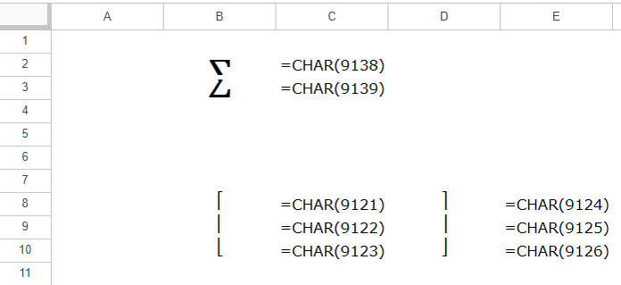

CHAR Function in QUERY

We can use the CHAR function within the QUERY function to filter a column that contains characters like checkmarks, crosses, and so on.

In the following example, I want to filter the individuals who have renewed their memberships. How can we identify them?

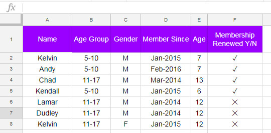
Observe the checkmark next to the names of those who have renewed their memberships. To filter them, you can either copy and paste the checkmark character within the formula or use the CHAR function.

Here’s an example using the CHAR function to filter based on the checkmark character in column F:

=QUERY(A2:F8,"SELECT * WHERE F='✓'")

If you know the table number of the checkmark in column F, you can use it as follows:

=QUERY(A2:F8,"SELECT * WHERE F="&" '"&CHAR(10003)&"' ")

Even if you don’t know the table number, you can find it using the CODE function in a QUERY formula, as shown here:

=QUERY(A2:F8,"SELECT * WHERE F="&" '"&CHAR(CODE(F2))&"' ")