You may sometimes want to freeze a cell in the source in Importrange to always point to a particular cell value.

So when the owner adds or removes rows and columns in the source, it won’t affect the imported value. It will move with the source cell.

Usually, locking a cell reference is not possible with Google Sheets Importrange function. But there are two workarounds.

You can freeze a cell in Importrange in Google Sheets using a Query or Named Ranges. Both aspects, I’m going to elaborate on this Google Sheets tutorial.

Lock a Cell Reference in Google Sheets Importrange – Why It’s Required?

Locking a cell reference or freezing a cell in Importrange is a must when we want to import only a specific cell value, usually a cell containing total or any aggregated value.

In this example, you can see that cell H13 contains the sum of values in the range H2:H12.

I can easily import this cell value into another worksheet.

Generic IMPORTRANGE Formula:

=IMPORTRANGE("spreadsheet_url","sheet_name!H13")

But the problem here is when I delete or insert any row between H2:H12 in the source sheet, the cell containing the total in H13 moves.

When you delete 1 row, it moves to H12. But our Importrange formula keeps importing the value from cell H13.

It’s because the IMPORTRANGE function uses range_string for importing data.

Syntax: IMPORTRANGE(spreadsheet_url, range_string)

How to Lock or Freeze a Cell in Importrange in Google Sheets

I’ve two options that you can consider to freeze a cell in Importrange in Google Sheets.

You can lock or freeze a cell in Importrange using QUERY or Named Ranges. Let’s go to that.

Using Named Ranges

Please see the above screenshot, where our total is in cell H13. It’s the sum of the range H2:H12.

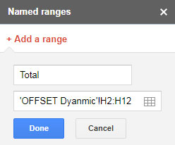
We should name cell H13. For that, go to the menu Data > Named Ranges.

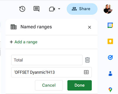
Name the Range “Total”

Note:- The name of my source sheet is “OFFSET Dyanamic”

Now open the sheet where you want to import the value of cell H13.

Apply the Importrange formula as below.

Formula 1:

=IMPORTRANGE("spreadsheet_url","Total")

It’s a generic formula. So, you may change the spreadsheet_url with the source Sheet URL.

This way, we can lock or freeze a cell reference in an Importrange formula.

Alternatively, you can name the range H2:H12 and sum the imported data.

Formula 2:

=SUM(IMPORTRANGE("spreadsheet_url","Total"))

Pros and Cons of Locking Cell Range in Importrange Using Named Ranges

Pros:

Formula 1 and Formula 2:

Adding or removing rows or columns in the Importrange source won’t affect the result.

The named range will automatically get adjusted and so you will get the correct cell value or cell range imported.

Cons:

Formula 2:

Any change in the SUM formula range in H13 won’t reflect in our above Formula 2 because we are importing H2:H12 and then summing it.

The below formula can handle this disadvantage.

Lock or Freeze a Cell in Importrange Using Query

Here is the second option to freeze a cell or cell range in Importrange in Google Sheets.

It is the recommended option and the most dynamic.

There is an additional requirement to make the below formula work. I’ll come to that.

I want to import the cell content in H13, i.e., SUM of H2:H12, into another sheet. But see the text in D13 below. Yes, it’s required.

You should place the text “Total” in row 13 in any text column (column containing texts only).

The suggested cells are A13, B13, D13, and E13. I opted for D13.

It’s an additional requirement to freeze cells using Query.

Now see the generic formula. You may replace the spreadsheet_url with your original URL.

=QUERY((IMPORTRANGE("spreadsheet_URL","OFFSET Dyanmic!A1:H")),"Select Col8 where Col4='Total'",0)

Don’t get confused. HereOFFSET Dyanmic!A1:H is the data range to import.

The above is the best formula to freeze a cell in Importrange in Google Sheets. Why? Just take a look at the Pros and Cons of this formula.

Similar: Offset Function Examples in Google Sheets and Dynamic Ranges

Pros:

No limitation, you can add or delete any rows. It won’t affect the locked cell.

Cons:

It uses a helper cell, i.e., D13, in the cell to lock in Importrange.

Deleting columns will affect the result.

This way you can freeze a cell in Importrange in Google Sheets.