Vlookup to Find Nth Occurrence in Google Sheets [Dynamic Lookup]

You are on the right page if you are searching for a way to perform a dynamic lookup in Google Sheets. Here is my complete solution to find Nth Occurrence in Google Sheets.

What more! You can use my formula on your Sheets without any issue.

No scripts were used to find the Nth occurrence. Only the Google Sheets built-in functions are used.

Understand What Is Nth Occurrence in a Vertical Lookup in Google Sheets

First of all, let me explain to you what is Nth occurrence of a search key in a dataset is.

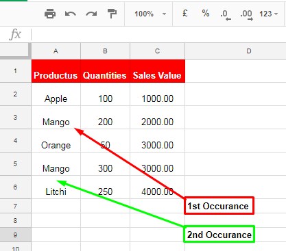
In the above screenshot, I have marked the 1st and 2nd occurrence of the item, “Mango.” I hope you have got the idea now. Here “Mango” is the search key.

To vertically search for a value and return another value from another cell (column) in the same row, we usually use the VLOOKUP function.

VLOOKUP is the blue-eyed boy of all spreadsheet users. No matter whether they are using Google Sheets or Microsoft Excel.

As a side note, Vertical Lookup means searching down in a column for an item.

Can We Use a Vlookup Formula to Vertically Lookup First, Second or Third Occurrence or Match?

In the usual way, it’s not possible. We can only use the VLOOKUP to return the first occurrence.

For example, the below Vlookup formula can find the first occurrence of the item “Mango” and return the corresponding value from the same row.

=VLOOKUP("MANGO",A2:C6,2,FALSE)

There is a better function in Google Sheets to do a vertical lookup.

It’s a combination of Match and Index Functions. It brings much dynamism for vertical and horizontal lookup in Google Sheets.

I have already explained how this Index-Match combo works as an alternative to Vlookup in Google Spreadsheets.

But, there, I didn’t mention this advanced part of vertical lookup, i.e., find Nth occurrence in Google Sheets.

To find the Nth occurrence in a vertical lookup, we can use different combinations of formulas.

How to Find Nth Occurrence in Google Sheets – Formula Options

You can find the Nth occurrence of a value (search key) in a vertical lookup using either of the below Google Sheets formulas.

INDEX, SMALL, ROW, ARRAY, and IF combo.
FILTER and INDEX combo.

Learn both of them or pick the combination that you think is easy for you to understand and use.

Once you complete this tutorial, you can do a vertical lookup using a search key and its 1st, 2nd, 3rd, or 4th occurrence or match.

INDEX, SMALL, ROW, ARRAY, and IF – A Killer Combination to Find Nth Occurrence in Vertical Lookup

I am going to use the above combination of formulas for our purpose.

I am directly going to the formula.

If you want to learn all these formulas individually, please check our ultimate Google Sheets Functions Guide.

Now to the example:

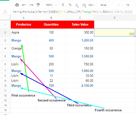
How to Find 1st, 2nd match in vlookup in Google Sheets

In the above screenshot, I’ve marked the first, second, third, and fourth occurrences of the item “Mango.”

Now see the below four formulas. The formulas will fetch values from the second column, i.e., under the field label “Quantities.”

=ARRAYFORMULA(IFERROR(INDEX(B2:B,SMALL(IF("MANGO"=A2:A,ROW(A2:A)-1),1))))
=ARRAYFORMULA(IFERROR(INDEX(B2:B,SMALL(IF("MANGO"=A2:A,ROW(A2:A)-1),2))))
=ARRAYFORMULA(IFERROR(INDEX(B2:B,SMALL(IF("MANGO"=A2:A,ROW(A2:A)-1),3))))
=ARRAYFORMULA(IFERROR(INDEX(B2:B,SMALL(IF("MANGO"=A2:A,ROW(A2:A)-1),4))))

Note:- The ARRAYFORMULA is optional as there is already INDEX (another array function) in use.

The first formula will search the range A2:A for the item “Mango” and return the value 400 from the same row in the second column.

The occurrence number is at the end of the formula. It decides which occurrence to be checked.

In the first formula, 1 means the first occurrence of the item “Mango.”

The second, third, and fourth formulas are the same. But the only difference is in the occurrence number.

So these formulas will fetch the values 500, 600, and 700, respectively ( from column 2).

How Can I Use This Dynamic Lookup Formula in My Spreadsheet to Find Nth Occurrence?

You can copy and paste the above formula and modify it. Please follow the below guidelines.

Change “Mango” in the formula part "MANGO"=A2:A with any other (search key) item based on your dataset. If the search key is in not in A2:A, replace A2:A too.
Change the Nth occurrence number in the formula. You can see the occurrence number at the end of it.
You should change this ROW(A2:A)-1 part of the formula based on your range. For example, If your range is A3:A, you should use this as ROW(A3:A)-2.
Change B2:B. I have used this range to return values based on the match found in A2:A.

Additional Notes:

This way, you can use my formula on your dataset.

But if you want to learn how I have coded the above formula, you should go through the below two tutorials.

Before that, please see once again the formula in use.

=ARRAYFORMULA(IFERROR(INDEX(B2:B,SMALL(IF("MANGO"=A2:A,ROW(A2:A)-1),1))))

1. Please check this Index formula tutorial for the pale pink part of the formula.

2. The vivid cyan blue part, I’ve already detailed in another tutorial. It’s Google Sheets SMALL+ROW formula combo.

Here is the second formula, which seems easy to learn, to Vlookup nth occurrence in Google Sheets.

Filter and Index to Return 1st, 2nd, 3rd, etc. Match in Google Sheets

Using the Filter function, we can filter rows containing our Vlookup criteria. It’s a straightforward formula, right?

=FILTER(A2:C,A2:A="Mango")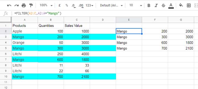

Now we can apply row and column offsets using Index.

For example, use the below formula to vertical lookup the second occurrence of the item “Mango” and return the “Sales Value” from the third column.

=index(FILTER(A2:C,A2:A="Mango"),2,3)

In this, 2 is the occurrence number, and 3 is the column from which we want the result to extract.

1st, 2nd, 3rd, and 4th Occurrence Formulas:

=index(FILTER(A2:C,A2:A="Mango"),1,3)
=index(FILTER(A2:C,A2:A="Mango"),2,3)
=index(FILTER(A2:C,A2:A="Mango"),3,3)
=index(FILTER(A2:C,A2:A="Mango"),4,3)

This way, you can successfully find Nth occurrence in Google Sheets.

I hope you have enjoyed this advanced Lookup tutorial in Google Sheets.

Thanks for the stay. Enjoy!

32 COMMENTS

Jorge Soria August 10, 2023 At 1:25 am

Hello Prashanth,

Thank you very much. The formula is retrieving all the matches from the same search key. I have a quick question: Is there any way to arrange the records in the same row where the search key is found? It can expand to 10 columns (I have that layout already).

- Prashanth August 10, 2023 At 9:18 am
  
  Yes! You can use the TOCOL function to make the output into a single column. Then, you can use the WRAPCOLS function to wrap the result into n columns.
  
  You can see a similar approach in Excel here. However, if you use that approach (formula), you will need to remove the DROP function. This may leave one blank row at the top of your result, but it will not cause any issues.
  
  If you would like any further assistance, please share a sample file URL (with Viewer access) below.
  
Jorge Soria August 8, 2023 At 2:29 am

Hi Prashant,

I came across your tutorial and it’s really helpful in retrieving information from a dataset I have. However, I’m stuck in a loop where everything I try only gets me the first matching records of the dataset.

I have this formula:

=ArrayFormula(IF(ROW(U:U)=1, "DATOS", IF(ISBLANK('P. ALBA 2023'!B:B), "", IFERROR(VLOOKUP(B:B, 'P. ALBA 2022'!C:Z, {8, 3, 9, 11, 10}, FALSE), "*"))))

This formula is capable of retrieving data from several columns in the row where a match is found. However, I want to populate additional columns as there are additional matches in the same dataset.

For example, let’s say I have a name in my search sheet, and that same name is recorded twice in the database (the P. ALBA 2022 sheet). What I want to do is to retrieve the same columns {8, 3, 9, 11, 10} for each match.

Do you have any suggestions on how I can do this?

- Prashanth August 8, 2023 At 8:21 am
  
  Hi Jorge Soria,
  
  VLOOKUP or XLOOKUP cannot retrieve multiple rows of matching records for the same search key.
  The function you can rely on is QUERY or FILTER with the REDUCE LHF.
  
  Please give this formula a try.
  
  =REDUCE({"DATOS","DATOS","DATOS","DATOS","DATOS"},TOCOL(B2:B,1), LAMBDA(accu,key,IFNA(VSTACK(accu,HSTACK(key,FILTER( CHOOSECOLS('P. ALBA 2022'!C:Z,{8, 3, 9, 11, 10}), 'P. ALBA 2022'!C:C=key))))))
  
  I hope this is helpful!
  
Shi Yu April 23, 2023 At 5:21 am

I appreciate this solution!

My data is spread across multiple columns that are non-repeating.

E.g.:

In the example below, 1-4 represents the list of colleagues in a team, and the fifth column represents the team leader.

If I would like to find out all the team leads that “JACK” has, what formula should I use?

A1 | A2 | A3 | A4 | team lead
JACK | albert | sally | roman | adam
jonas | rocky | gene | chris | alex
John | JACK | William | Robert | eve

- Prashanth April 25, 2023 At 10:21 am
  
  Hi, Shi Yu,
  
  There are several ways to achieve this. One way to do this is using the below formula in cell F2.
  
  I assume the range is A1:E where A1:E1 contains the headers.
  
  =textjoin(", ",1,unique(tocol(bycol(A2:E,lambda(c,ifna(filter(E2:E,c="Jack")))))))
  
andrei December 26, 2022 At 5:36 am

Is it possible to make an out-of-range occurrence return nothing?

In your example, the 4th occurrence of Litchi would return values for the last mango.

- Prashanth December 27, 2022 At 2:33 pm
  
  Hi, Andrei,
  
  Sorry, I could not replicate that issue within my Sheet. I suggest you share your example Sheet.
  
Nick Johns December 19, 2022 At 7:01 am

Hello, this worked great for me! Thank you. But is there any way to add a second criteria column?

I want to look up all invoices that match the customer ID and then also check those against the “Status” column to see that it is paid.

I tried combining the criteria in this formula, but it didn’t work.

=IFERROR(INDEX(Invoices!C$2:C,LARGE(IF(and((isnumber(find("Paid", Invoices!E$2:E))=FALSE),Invoices!B$2:B=C3), ROW(Invoices!$B$2:$B)-1),1)))

Any help is MUCH appreciated. Again, thanks for the helpful article!!!

- Prashanth December 19, 2022 At 12:09 pm
  
  Hi, Nick Johns,
  
  I assume Invoice!B2:B contains invoice numbers, and Invoice!E2:E is the status column.
  
  To filter Invoice!C2:C if Invoice!B2:B=C3 and Invoice!E2:E contains “Paid”, use the following filter.
  
  =filter(Invoices!C2:C,Invoices!B2:B=C3,regexmatch(Invoices!E2:E,"Paid"))
  
  It will return a multi-row output. You can use Index to offset rows and get the nth value.
  
  E.g.:
  
  =index(filter(Invoices!C2:C,Invoices!B2:B=C3,regexmatch(Invoices!E2:E,"Paid")),3)
  
Dale Harper August 22, 2022 At 11:57 pm

Hi, This has been an absolute lifesaver! Does this work with Hlookup?

- Prashanth August 23, 2022 At 9:37 am
  
  Hi, Dale Harper,
  
  Yep! But you may require to slightly adjust the formula.
  
  I’ll update you soon!
  
Irving Beltran April 18, 2021 At 3:52 am

Hi,

I hope you’re doing well. I used your formula, and it works great for finding the first two occurrences of an item. But it just won’t work for the 3rd, 4th, and 5th occurrences. This is my modified formula:

=INDEX(filter(A2:AB,((B2:B=AK2))*((AB2:AB="No recibido"))),3,28)

I get an error message that says, “The second parameter is 3. Valid values must be between 0 and 2.” Could you please help me find a way to bypass this parameter restriction?

- Prashanth April 19, 2021 At 8:41 am
  
  Hi, Irving Beltran,
  
  You will see that error when there is no third occurrence.
  
  You might want to use the OR condition in FILTER.
  
  =index(filter(A2:AB,((B2:B=AK2)+(AB2:AB="No recibido"))),3,28)
  
  This may help – How to Use AND, OR with Google Sheets Filter Function – Advanced Use.
  
  - Irving Beltran April 19, 2021 At 8:00 pm
    
    Hi,
    
    Thanks for your quick response. I was able to fix my formula by clicking on the link you sent me and by learning a bit more from other sections on your site. Keep up the awesome work! Godspeed!
    
David Austin January 9, 2021 At 11:10 pm

Hi, I’m a bit of a beginner but the formula worked really well. I wanted all the nth occurrences in my spreadsheet added together so I just did the formula with a plus sign and then the formula again with the next occurrence and repeated over and over again like this:

=ARRAYFORMULA(IFERROR(INDEX($Q$3:$Q,SMALL(IF($S$3=$P$3:$P,ROW($P$2:$P)-1),1))))+(IFERROR(INDEX($Q$3:$Q,SMALL(IF($S$3=$P$3:$P,ROW($P$2:$P)-1),2))))

This worked but I guess it’s not the proper way to do it. What is?

Thanks again

- Prashanth January 12, 2021 At 8:03 am
  
  Hi, David Austin,
  
  I think I can solve this. Can you please leave the URL of a sample sheet in your reply?
  
Sandra August 10, 2020 At 11:56 pm

I want to be able to do this on a separate sheet. That is, I have collected form responses and I created a new sheet. I want to lookup responses and have the formulate populate the answers to Vlookup in the new sheet. What would the new formula look like?

- Prashanth August 11, 2020 At 12:33 pm
  
  Hi, Sandra,
  
  You have not given the data range or enough information. When you say a new sheet, were you referring to a new file or a new tab in the same form response sheet?
  
Will March 17, 2020 At 10:20 pm

Nice formula!

If I want to use it without the INDEX, and just have it return the ROW numbers, can it be made into an Array Formula?

Thank you

- Will March 17, 2020 At 11:03 pm
  
  In fact, I wouldn’t need SMALL either as I want all the row numbers that meet the criteria. This formula produces an array ARRAYFORMULA(IF(value=range,ROW(A1:A))) I get a long list of FALSE with the occasional ROW number interspersed. My question now is – how do I show a list with just the ROW numbers?
  
  Thank you
  
  - Will March 17, 2020 At 11:44 pm
    
    FILTER and ISNUMBER seem to work!
    
    - Prashanth March 18, 2020 At 11:19 am
      
      Hi, Will,
      
      No need to use the IF test. You can directly use Filte or Query.
      
      Can you show me a demo of your problem by sharing an example sheet? I may be able to help you.
      
Peter Kruger November 20, 2019 At 9:47 am

Is this still working? When I applied it to my sheet, it gave me a formula parse error so I fully recreated your sheet exactly and copy and pasted your formula and got the same error. Any advice?

- Prashanth November 21, 2019 At 4:55 pm
  
  Hi Peter,
  
  Once copy-paste, re-type the double quotation marks. It causes issues in copy-paste.
  
  Best,
  
AJ September 20, 2018 At 11:19 pm

I really appreciate this, it was very helpful and clearly laid out. One question: is the “ArrayFormula” necessary? I tried it without “ArrayFormula” and it still seems to work. I am fairly new to using “ArrayFormula” and am looking to learn more. I figured I would inquire what purpose it serves in this formula.

- Prashanth September 21, 2018 At 8:17 am
  
  Hi, AJ,
  
  I am glad to hear that you liked this tutorial on Nth occurrence!
  
  Now regarding your question, use the ArrayFormula function with non-array functions.
  
  For example, in our formula that finds Nth occurrence in Google Sheets, I have used the function ROW in a range (array). The ROW is a non-array function. So I’ve used the ArrayFormula.
  
  But there are certain Exceptions. If you use a non-array function, here example the ROW function, within an array formula like FILTER or INDEX, there is no need to again use the ArrayFormula. Here Index itself is an array formula.
  
  So ArrayFormula is not a must here.
  
  I have used the ArrayFormula to avoid the confusion.
  
  Thanks.
  
Ken Snyder September 1, 2018 At 6:28 am

Very good stuff. I really like using named-ranges for things and instead of the A2:A,ROW(A2:A)-1 in the example I’m wondering how I could get this to work. I have a named range called PEOPLE_NAMES which is a column of names.

- Prashanth September 1, 2018 At 8:57 am
  
  Hi,
  
  You can use named ranges. But not advisable as you may require to use Query to extract individual columns from the multiple columns named range.
  
Tim Watson August 31, 2018 At 2:35 am

This is great! Only trouble for me is that the arrayformula isn’t populating down the page (just showing result in the cell where the formula is). Any advice?

- Prashanth August 31, 2018 At 7:00 am
  
  Hi, Tim,
  
  I am glad that you liked it.
  
  Regarding expanding result, I think it’s not possible because of the use of INDEX which doesn’t support.
  
RSigu January 31, 2018 At 7:11 pm

It Worked like a charm!!! Thank you!!! 🙂