


There are many formulas to find the minimum value in a column and return the corresponding value from another column in Google Sheets. In this post, I will show you how to use the INDEX-MATCH-MIN combo to do this.
As you may know, the MIN function can return the minimum value from a numeric data set. However, can we use the MIN to return values from adjacent cells other than the minimum value?
No, we can’t. But, we can use it with the lookup functions for the same.
I am referring to a vertical lookup where the search key is the smallest value in the column. First, we need to find the smallest value to use in the lookup and the MIN will take care of that.
We can also offset the min value row number in an adjacent column using INDEX.
Let’s see how to find the minimum value and return a value from another column in Google Sheets.
Lookup or Find Minimum Value and Return Value From Another Column
Sample Data and MIN formula:
The following sample data contains the names of a few people and their ages.
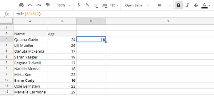
The following MIN formula in cell C3 returns the minimum value, or smallest value, in the numeric column B.
=MIN(B3:B12)The value 16 is the age of the person “Erinn Cady,” and that name is in column A. Can we look up column B for the minimum age and return the name from column A?
Yes, we can do that. You may think that you can use VLOOKUP for this purpose. But the problem here is, VLOOKUP looks at the first column for a match and returns the corresponding value from another column. So a kind of Reverse VLOOKUP we want here.
Our lookup value is in column B and we want to return the result from column A. Further to deepen the problem, we don’t have the search key or minimum value in hand to use directly in the lookup.
So the solution is an INDEX, MATCH, and, MIN combo formula. With this killer combination of functions, we can find the minimum value in Google Sheets and return values from another column.
Sure, we can use reverse VLOOKUP too. However, I am opting for the combination I mentioned as it will be easy for people who are familiar with Excel (switched to Google Sheets from Excel).
The MIN Function in Vertical Reverse Lookup (INDEX-MATCH)
Below is the popular combination formula for the type of lookup that I am talking about.
=INDEX(A3:A12,MATCH(MIN(B3:B12),B3:B12,FALSE),1)Syntax:
INDEX(reference, [row], [column])I have compared the INDEX function’s parameters with our combo formula’s arguments, using different colors to distinguish them.
The “row” part (in blue color) in the INDEX is the key in this combo formula.
If we have the row number of the smallest value, we can easily return the name of the person by using the INDEX function with that row number as the row parameter.
In the absence of the row number, I have used a MATCH and MIN combination to return the row number, as shown below.
MATCH(MIN(B3:B12),B3:B12,FALSE)See the MATCH syntax now.
MATCH(SEARCH_KEY, RANGE, [SEARCH_TYPE])The Role of MIN in the MATCH-MIN Combo:
The MIN function in the combo formula returns the smallest value in column B.
The Role of MATCH in the MATCH-MIN Combo:
The MATCH formula uses this number as “search_key” to return the relative position of the number which is the row number.
This way, you can find the minimum value and return value from another column in Google Sheets.
Alternative Solutions to Find the Min Value and Return Value from Adjacent Cell
Here are some popular alternatives to finding the minimum value and returning the value from an adjacent cell in Google Sheets.
1. XLOOKUP.
=XLOOKUP(MIN(B3:B12),B3:B12,A3:A12)2. FILTER (Useful when you have more than one min value).
=FILTER(A3:A12,B3:B12=MIN(B3:B12))3. Reverse VLOOKUP.
=VLOOKUP(MIN(B3:B12),HSTACK(B3:B12,A3:A12),2,0)That’s all.
Hi! I am trying to do this, but the minimum value is across multiple rows and columns. How do you do this when you are looking for a minimum value in a range of cells between B2:D500?
Hi Ryan,
I assume you want to return a value from A2:A500 that corresponds to the minimum value in B2:D500.
You can use the following formula as the row argument in the INDEX function:
TOROW(BYCOL(B2:D500,LAMBDA(col,MATCH(MIN(B2:D500),col,FALSE))),3)This is great! I’m using this to create a scoreboard for the popular game “Wordle.”
I used this particular formula to create rankings, but I’m having trouble displaying it properly when there are ties.
You can view the sheet below. The cells I’m using the formulas are T3 – T15.
– link removed —
Hi, Tyler,
You have got user names in B1:N1 and corresponding averages in B31:N31.
Make an array of these two rows, transpose, and sort. You can use the below formula for that.
=sort(transpose({B1:N1;B31:N31}),2,1)I have this in range T3:U15 (above formula in T3).
Then find the rank of column 2 of this array. For that, use the following RANK formula in V3.
=ArrayFormula(rank(U3:U15,U3:U15,1))Added to tab “prashanth” in your Sheet.
Amazing! Thank you for being a Google Sheets wizard.
Is there a way to only have it output numbers greater than 0.
For example, I have 2 columns with section times and a 3rd that gives the totals of those 2 sections.
Since not all people completed both sections I have a formula in the 3rd column that returns a 0 for those with a blank time.
Then I want to sort the 3rd column for the lowest actual time for both sections.
There are several methods to conditionally find a min value greater than 0.
If your said data range is A2:C, then you can try the below FILTER and SORTN combination formula.
To only return the min value row excluding 0.
=sortn(filter(A2:C,C2:C>0),1,0,3,1)To return the data sorted in descending order but only values greater than 0
=sortn(filter(A2:C,C2:C>0),9^9,0,3,1)Here is a related guide – How to Exclude 0 From MIN Function Result in Google Sheets.
Is there a way for it to output 2+ if there is a tie?
Hi, Carter,
Use the filter.
=filter(A3:B12,B3:B12=min(B3:B12))Best,
Thank you for sharing your knowledge and expanding mine.
I like your article(s) very much.
But still, I would like to ask you if there’s a misspelling in the title(s) “the Roll of MIN…”?
Did you mean to say “the Role”, and not “roll”, because “Role” would make more sense to me?
Thank you again.
Sorry for the typo!
It’s happy to know that you like my tutorials.