Do you know how to filter data for a certain number of weeks in Google Sheets like 1 week, 2 weeks, 3 weeks etc.? If not, this tutorial is for you. I am going to provide you a very flexible formula for this purpose. You can modify and use this custom filter formula for your purpose.
In Google Doc Spreadsheet, there are two options to filter data using the number of weeks as the condition. They are QUERY and FILTER.
In this Google Sheets tutorial, I’m going to use the FILTER function as it’s very simple compared to QUERY in terms of handling the date criteria. Using date criteria in Query is tough to follow.
How to Filter Data for Certain Number of Weeks in Google Sheets
This time I’m not posting a screenshot of my sample data as it’s too long. It’s like this.
Cell range A1: A31 contains the date from 01/10/2017 to 31/10/2017 in progressive or chronological order. The corresponding column range B1: B31 contain some random numbers. You can put any data in this range as it’s not important or not be going to affect our tutorial purpose.
That’s all. It’s a two column data where we are using our above filter tricks.
We are going to filter the last two weeks data from the above data range and I’ve considered the weeks are from Monday to Sunday.
The Formula to Filter Data for Certain Number of Weeks
Scenario # 1
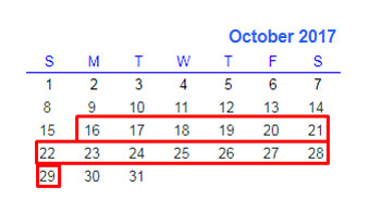
Our starting date as per the sample data is 01/10/2017 and the end date is 31/10/2017. If you consider Monday to Sunday as the week starting and the week-ending dates, the perfect filtered data would be with in the below date ranges.

Formula:
=filter(A1:B,A1:A>=(max(A1:A)-(weekday(max(A1:A),2))+1)-2*7,A1:A<=(max(A1:A)-(WEEKDAY(max(A1:A)))+1))
When you use this formula to filter data for a certain number of weeks in Google Sheets note the following points.
1. Here the data range is A1: B You can change it as per your data range like A1: E or A1: F etc.
2. The above Filter formula will filter the data for last two weeks. If you want to change the number of weeks, see the 2*7 multiplication part in the formula. When you change 2*7 to 5*7 it considers as 5 weeks and accordingly the filter would happen.
The same is applicable to Scenario # 2 and Scenario #3 below. How to develop this filter formula then? I know you are curious about it. I will tell you that part at the end of this post.
Scenario # 2
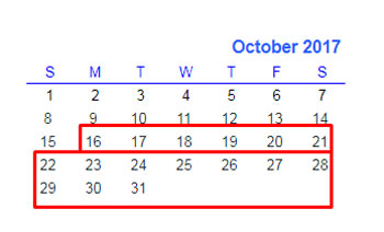
Here in this scenario, I’ve considered the last two weeks as below. Here the filtering we are going to apply from the most recent date in our data, i.e., 31/10/2017 to two weeks back.

Formula:
=filter(A1:B,A1:A>=(max(A1:A)-(weekday(max(A1:A),2))+1)-2*7,A1:A<=(max(A1:A)))
Every point that I’ve mentioned under Scenario # 1 is applicable here also.
Scenario # 3
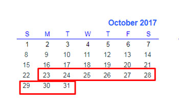
Here you can guess what is the two weeks range. Its’ the most recent half week + past one week.

Formula:
=filter(A1:B,A1:A>=(max(A1:A)-(weekday(max(A1:A),2))+1)-1*7,A1:A<=(max(A1:A)))
This is the same formula as Scenario # 2. But only one difference is here. In Scenario # 1 and Scenario # 2, the multiplication part in the formula is 2*7. Here it’s 1*7.
That means when you want to filter 5 weeks data, in this last formula, you should put 4*7. But in the first and second formula, it should be 5*7.
Conclusion:
If you know how to use the FILTER formula in Google Sheets, then you may only want to know one thing with the above formulas.
That is, how to find last certain number of weeks. That part, I’ve detailed in a separate post Here. Hope you find this Filter Data for Certain Number of Weeks in Google Sheets tutorial useful. Enjoy!


