Understanding why the EXACT function in Google Sheets is important is essential before learning how to use it.

The EXACT function primarily revolves around case sensitivity. The majority of spreadsheet functions are case-insensitive.

This underscores the significance of the EXACT function in Google Sheets.

What Functions in Google Sheets Are Case Insensitive?

I won’t list each function individually regarding case sensitivity.

In general, most functions in Google Sheets are case-insensitive. However, exceptions include functions like UNIQUE, QUERY, EXACT, FIND, REGEXREPLACE, REGEXMATCH, and REGEXEXTRACT, which are case-sensitive.

For functions involving regular expressions, such as the ones mentioned above, you can use the (?i) modifier to ignore case sensitivity.

Example:

=REGEXMATCH(F4,"(?i)apple")

The formula will return TRUE if “apple” (case-insensitive) is found in the text in cell F4 and FALSE otherwise.

EXACT Function: Syntax and Arguments in Google Sheets

Let’s start with the syntax of the EXACT function:

Syntax:

EXACT(string1, string2)

Arguments:

• string1: The first string to compare.
• string2: The second string to compare.

Purpose:

The EXACT function checks two strings for exact matches, including identical cases, spaces, or hidden characters, and returns TRUE or FALSE.

Examples of How to Use the EXACT Function in Google Sheets

Here are two formulas:

=EXACT("apple", "APPLE") // returns FALSE
=EXACT("APPLE", "APPLE") // returns TRUE

The first formula returns FALSE because both strings are not identical. The first string is the text “apple” in lowercase, whereas the second string is the same text but in uppercase letters.

For further illustration of the EXACT function in Google Sheets, I’ve copied and pasted the following formula from cell D2 to D7 to compare each value in column A with its corresponding value in column B:

=EXACT(A2, B2)

Some Clever Applications of the EXACT Formula

In the above example, the formula in row #4 returns FALSE as the value in cell A4 contains an extra space. In such cases, you can use the TRIM function within the EXACT function as shown below:

=EXACT(TRIM(A4), B4)

Similarly, observe how I use the EXACT function in a simple logical test with the IF statement.

Take a look at row #3 in the above example, which returns TRUE. The following logical test would return the string “perfectly matching” instead of the TRUE boolean value.

=IF(EXACT(A3, B3), "perfectly matching!")

This demonstrates the versatility of the EXACT function in various scenarios within Google Sheets.

How to Convert a Case-Insensitive Formula to a Case-Sensitive?

In most cases, you can employ the REGEXMATCH function to fulfill your case-sensitive formula requirement. However, the EXACT function can also be used.

For instance, if you want to count the occurrences of a particular case-sensitive ID, “XYZ”, in the cell range B2:B, the following COUNTIFS formula will return the case-insensitive count:

=COUNTIFS(B2:B, "XYZ")

To obtain the case-sensitive count, you can enter the following EXACT array formula in cell C2:

=ArrayFormula(EXACT(B2:B, "XYZ"))

Then, use the following COUNTIFS:

=COUNTIFS(B2:B, "XYZ", C2:C, TRUE)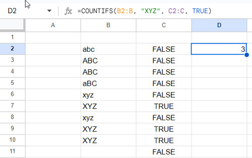

Related Reading:

1. How to Do a Case Sensitive Sumproduct in Google Sheets.
2. Case Sensitive Reverse Vlookup Using Index Match in Google Sheets.
3. How to Perform a Case Sensitive COUNTIF in Google Sheets.
4. How to Do a Case Sensitive SUMIF in Google Sheets.
5. Case Sensitive Vlookup in Google Sheets.
6. How to Do a Case Sensitive DSUM in Google Sheets.
7. How the EXACT Function Differs in Excel and Google Sheets.