


")


Here you can learn a unique way of creating DYNAMIC RANGES in Google Sheets. It’s possible to create Dynamic Ranges in Google Sheets without Helper Cell.
By saying Helper Cell, I mean to say the formula itself can handle dynamic ranges without referring to any additional cell or column.
Similar: Virtual Helper Column in Google Doc Spreadsheets.
This is a combination of functions that make your ranges in the formula always dynamic. You just set and leave dynamic ranges in your SUM, SUMIF, SUMIFS, COUNTIF, MAX, MIN, or any formulas accepting column ranges.
Later you can add or remove any number of rows in your data, that will automatically be adjusted in the range. Dynamic Ranges in Google Sheets without helper cells is a reality.
Must Read: Google Sheets Functions Guide (learn all Google Sheets most useful functions).
I have earlier explained how to create a dynamic range using OFFSET function in Google Sheets. What’s the difference between that formula with this new one?
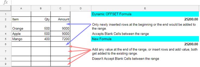
Dynamic Offset Formula Vs the New Formula (Quick Comparison)
Both have plus and minuses. Here is that comparison.
Screenshot # 1:
Before Going to this new and fresh dynamic range tutorial, you may please go to my following tutorials to understand the main functions in use in this new formula. They are INDIRECT and ADDRESS. This will help you to read my formula better.
Creating Dynamic Ranges in Google Sheets Without Helper Cell (The Ultimate Way)
The below Dynamic Range formula would only consider existing values in a column range and automatically modify the range when you add new values at the end of the existing values. In other words, the dynamic range ends when a blank cell appears in the column.
The benefit of using a dynamic range is that you have always additional room in your Spreadsheet below your existing data range.
If you use an infinite range like G2:G or G:G in a formula, you can’t use the blank cells below for some other purposes.
You only need to just skip one row and keep that row always blank. You can use the rest of the rows for other purposes.
Now it’s time to go to the formula.
Similar: How to Use Dynamic Ranges in SUMIF Formula in Google Sheets (Using Offset function)
Here is our New Formula and sample Data. I am using the dynamic ranges in SUM function here.
The formula seems complex. But it’s not so. You can use it out of the box.
Screenshot # 2:
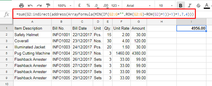
Dynamic Range Formula in Google Sheets Without Referring Helper Cell
Before explaining how to create the above dynamic range formula, let me tell you how you can use it.
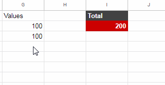
The above formula Sums column G. You can enter any values in the cells G10, G11, G12 and so on. It would get added to the SUM range.
If any blank cells appear in this column, the formula would return the wrong answer. Because the formula only sums up to that range only.
If you insert a row in between the range, remember to at least leave the value 0 in the corresponding column in use (column G here). Please keep this in mind if you use my formula.
Screenshot # 3:
Formula Explanation:
You can copy my below dynamic range formula.
Formula:
=sum(G2:indirect(address(ArrayFormula(MIN(IF(G2:G="",ROW(G2:G)-ROW(G2)+1))),7,4)))Here, G2 is the cell address of the beginning of the range. It can be any cell address in any column based on your data range.
Here are the details on how I have coded the above awesome formula.
=ArrayFormula(MIN(IF(G2:G="",ROW(G2:G)-ROW(G2)+1)It counts the range G2:G until any blank cell appears. I have detailed this formula in a separate tutorial. See the link just below this formula explanation part.
This formula just returns the value 9. Please refer the screenshot # 2 for the sample data and pay your special attention to column G. If you use normal Count formula, the result would be 8 only. The above formula returns count + 1.
When this formula wrapped by an Address formula, it would be like this;
=address(9,7,4)Here you must replace 9 with the above count formula.
=address(ArrayFormula(MIN(IF(G2:G="",ROW(G2:G)-ROW(G2)+1))),7,4)This address formula returns the cell address G9. Here 7 is the column number of G and 4 is the ‘absolute_relative_mode’ in the Address function.
The final formula is like;
=sum(G2:indirect(G9)In this G9 is the just above Address formula.
How to Count Until a Blank Row in Google Sheets
How Can I Use this Dynamic Range in My Own Sheet?
I know you may want to use this formula in a column other than G. If so, here is the only thing you may want to change.
In the formula, just change;
- G2 – Change this cell address to your starting cell address in the range.
- G– It goes without saying.
- 7 – This’s the column number of G. Column number for A =1, B=2… and G=7. Change it accordingly.
Finally, you can use the above dynamic ranges in Google Sheets in formulas other than SUM.
Do remember that we haven’t used any helper cell or column to create this dynamic range. That’s the beauty of this formula.
Use it only by understanding its limited drawback in handling blank cells. That’s all for now. Enjoy!
Access My Google Sheet Here to see the formula in action.
I love this solution, but I wonder if I can apply this to make a dynamic drop-down list.
Case in point: Whenever I enter a new transaction, I will select the right spending category from a drop-down list.
The data range where this list pulls from may get expanded in the future when I want to add a new spending category.
How should I do that?
Can you explain further or share a sheet with some explanation to the problem and sample data?
Hi, Trang,
In Sheets data validation you can use open ranges like A2:A. You are not restricted to limited ranges like A2:A9. I think this is not the case in Excel (I’ve left ‘regularly’ using Excel long back. So I’m unsure about the same in Excel).
Thank you, I’ve forgotten about that simple trick.
HELLO,
I just did a little modification to work in my case that the data start at the 6th row.
=SUM(E6:indirect(address(ArrayFormula(MIN(IF(E6:E="",ROW(E6:E)-1))),COLUMN(E5),4)))I hope that will be useful for somebody else!