Differences Between SUMIFS and SUMPRODUCT in Google Sheets

Although we can substitute SUMIFS with SUMPRODUCT in many cases in Google Sheets, the purposes of both functions are distinct.

There is a significant difference between the SUMIFS and SUMPRODUCT functions in Google Sheets. The former is a conditional SUM function, whereas the latter is designed to calculate the sum of products in two or more equally sized arrays. However, you can similarly utilize them.

When it comes to choosing between these functions for conditional sum, determining which one is better depends on your specific requirements. To find the answer to this question, explore the pros and cons of both SUMIFS and SUMPRODUCT outlined below.

Syntaxes:

SUMIFS: SUMIFS(sum_range, criteria_range1, criterion1, [criteria_range2, …], [criterion2, …])

SUMPRODUCT: SUMPRODUCT(array1, [array2, …])

Differences Between SUMIFS and SUMPRODUCT Functions

Below, I outline the key distinctions between SUMIFS and SUMPRODUCT in Google Sheets. It’s important to note that there is no official documentation available on this subject.

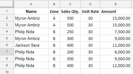
Consider the sample data in A1:E9, where columns A to E contain Name, Zone, Sales Quantity, Unit Rate, and Amount, respectively. Let’s use SUMIFS and SUMPRODUCT to conditionally calculate the total sales amount.

Sample data illustrating the distinctions between SUMIFS and SUMPRODUCT functions in Google Sheets

SUMIFS vs. SUMPRODUCT for Conditional Summation

Let’s calculate the total sales amount for “Philip Nida.”

SUMPRODUCT calculates the sum of products directly, eliminating the need to calculate the product (Sales Quantity * Unit Rate) separately in column E.

=SUMPRODUCT((A2:A9="Philip Nida")*C2:C9*D2:D9) // returns 34,500.00

Meanwhile, SUMIFS can sum the range E2:E9 using the condition.

=SUMIFS(E2:E9, A2:A9, "Philip Nida") // returns 34,500.00

In summary, use SUMPRODUCT when you don’t need the product of each item; otherwise, opt for SUMIFS.

Handling of Text Values in Numeric Fields

SUMIFS uses a logical approach, while SUMPRODUCT involves mathematical operations. Consequently, if there is a text value in the sum range, the former skips it, while the latter returns an error.

SUMIFS effectively ignores any non-numeric entries in the sum range, treating them as zero in the summation process.

Difference in Criteria Specification

DATE and number criteria are specified slightly differently in SUMIFS and SUMPRODUCT. Here is how to use the date criterion in these functions.

Date criterion in SUMIFS:

">="&DATE(2017, 7, 1)

Date criterion format in SUMPRODUCT:

>=DATE(2017, 7, 1)

Faster Processing

SUMIFS is reputed to be faster when used for its core purpose of conditional sum. It efficiently checks multiple ranges for provided conditions and returns the result.

ArrayFormula Function Support

When employing a value expression rather than a physical range in the criteria range of SUMIFS, it’s necessary to encapsulate the formula with the ArrayFormula function. An example illustrating this is provided later in the tutorial below. In contrast, SUMPRODUCT can autonomously handle logical calculations.

These are the main differences between the SUMIFS and SUMPRODUCT functions in Google Sheets.

When to Use the SUMPRODUCT Function in Google Sheets?

The primary purpose of the SUMPRODUCT function is to calculate the sum of the products of corresponding components in two equal-sized arrays or ranges.

It is essential to use the SUMPRODUCT function with this purpose in mind. The function is versatile, allowing the inclusion of criteria, which provides flexibility similar to the SUMIFS function.

When to Use the SUMIFS Function in Google Sheets?

The SUMIFS function is ideal when you need to calculate the sum of a range based on multiple conditions in different ranges.

Why do People Tend to Use SUMPRODUCT Over SUMIFS?

People tend to favor SUMPRODUCT over SUMIFS, especially when dealing with complex criteria for conditional sums.

For instance, consider the following data in columns A to D (Sales Date, Salesperson, Area, and Amount).

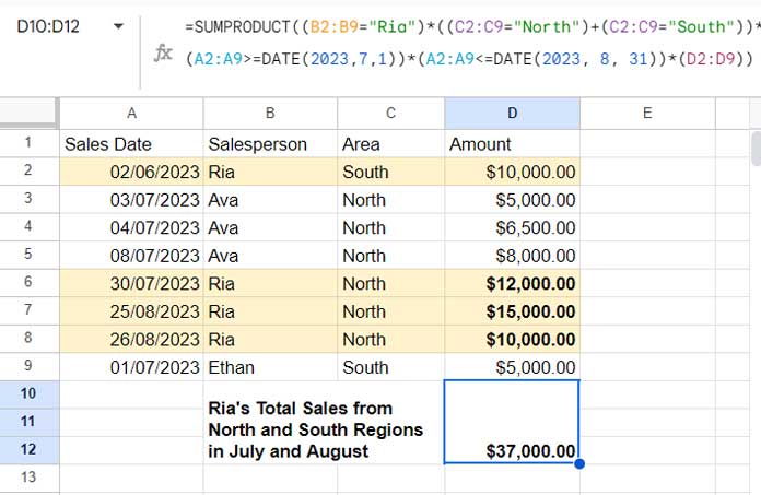
Ria's Total Sales from North and South Regions in July and August

To determine the total sales by “Ria” (Salesperson) in the “North” and “South” areas between 01/07/2023 and 31/08/2023, we can use the following SUMIFS formula:

=ArrayFormula(SUMIFS(D2:D9, (C2:C9="North")+(C2:C9="South"), 1, B2:B9, "Ria", A2:A9, ">="&DATE(2023, 7, 1), A2:A9, "<="&DATE(2023, 8, 31)))

Alternatively, the SUMPRODUCT formula provides a more concise approach:

=SUMPRODUCT((B2:B9="Ria")*((C2:C9="North")+(C2:C9="South"))*(A2:A9>=DATE(2023, 7, 1))*(A2:A9<=DATE(2023, 8, 31))*(D2:D9))

Note that in the SUMIFS criteria range, logical operations are employed, and as a result, faster performance may be compromised. In contrast, the SUMPRODUCT formula appears more organized and reader-friendly.

Resources

We’ve delved into the differences between the SUMIFS and SUMPRODUCT functions in Google Sheets, along with their use cases.

Here are additional resources related to these two functions.

Differences Between SUMIFS and SUMPRODUCT Functions in Google Sheets