What are the differences between SUMIFS and DSUM, the conditional sum functions, in Google Sheets? Let’s explore.

Typically, I create formulas specifically for Google Sheets users, but many of them are also applicable to Excel users. The “key differences” discussed in this tutorial are applicable to Excel as well.

I’ve already compared some differences in the functions of these two programs, which you can find here – Excel vs Sheets. Now, let’s return to our ‘conditional sum’ comparison tutorial.

In this post, I will explain the difference between SUMIFS and DSUM in Google Sheets and then elaborate on it with the help of a simple and easy-to-follow example.

You might wonder why I’ve skipped SUMIF, another function similar to SUMIFS and DSUM. The reason is simple.

The functions SUMIFS and DSUM can handle multiple criteria columns, whereas SUMIF is typically designed for a single criteria column.

I’ve already shared my unique tips for including multiple conditions in the SUMIF function here – Multiple Criteria Sumif Formula in Google Sheets.

SUMIFS and DSUM Key Differences in Google Sheets

Let’s begin by exploring the distinctions between SUMIFS and DSUM before delving into an example.

From my perspective, there are four major differences. Here they are:

1. Application:

• The DSUM function requires table-like structured data. It identifies the criteria range using field labels and the sum range using either field labels or column indexes.
• SUMIFS uses range references, eliminating the need for row headers (field labels). You must include the column ranges individually in the formula, not as a whole. This allows scattered criteria columns to be included in SUMIFS if they have the same number of rows.

2. Specifying Criteria:

• In DSUM, the criteria should be specified as a table with a header row containing field labels and criteria listed below. This can be complex if you want to hardcode the criteria. You must be familiar with creating arrays using either curly braces or VSTACK / HSTACK for this.
• In SUMIFS, you can specify the criterion as cell references or hardcode it within the formula.

3. Readability:

• A DSUM formula with multiple criteria is more reader-friendly compared to SUMIFS due to the clarity achieved by specifying criteria as a table.

4. Advanced Capability:

• Before the introduction of Lambda, advanced users utilized database functions for row-wise array formulas such as MIN, MAX, etc., by row. You can find a few examples under the tag “row-wise array.” This operation is not possible using SUMIFS.

Formulas to Make You Understand the Difference Between SUMIFS and DSUM

The following example aims to illustrate the distinction between the aforementioned two functions.

I may not delve into the detailed explanation of the formulas. For that, please refer to my function guide and select the relevant functions.

Sample Data and Criteria

Sample Data:

Below (please refer to the screenshot), I have structured data in the range A6:D14. The header row A6:D6 contains field labels: Name of Sales Person, Area, Sales Date, and Sales Value, respectively.

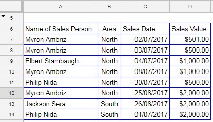
From the provided data, I will sum the “Sales Value” in column D for “Philip Nida” in column A based on the following conditions:

• Area: North or South (column B)
• Sales Date: Between 01/07/2017 to 31/07/2017 (column C).

First, observe the DSUM criteria and DSUM formula below.

Criteria Usage in DSUM:

See the criteria table in cell range A2:D4 in the screenshot below.

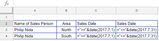
Note: In the range C3:D4, you won’t find the entered criteria as above. For example, after entering the criteria =">="&DATE(2017,7,1) in cell C3, it would be converted to >=42917. This is quite natural. You can read more about DSUM date condition use here – How to Use Date Difference As Criteria in DSUM in Google Sheets.

SUMIFS and DSUM Formulas

The DSUM Formula, as per the Syntax DSUM(database, field, criteria):

=DSUM(A6:D14, 4, A2:D4)

Where:

• database: A6:D14 (structured table)
• field: 4 (sum range)
• criteria: A2:D4 (criteria entered as a structured table)

The SUMIFS Formula, as per the Syntax SUMIFS(sum_range, criteria_range1, criterion1, [criteria_range2, …], [criterion2, …]):

=SUMIFS(D7:D14, A7:A14, A3, B7:B14, B3, C7:C14, C3, C7:C14, D3) + SUMIFS(D7:D14, A7:A14, A3, B7:B14, B4, C7:C14, C3, C7:C14, D3)

Where:

• sum_range: D7:D14
• criteria_range1: A7:A14
• criterion1: A3
• criteria_range2: B7:B14
• criterion2: B3 in first formula / B4 in second formula
• criteria_range3: C7:C14
• criterion3: C3
• criteria_range4: C7:C14
• criterion4: D3

Compared to DSUM, the SUMIFS formula is quite lengthy and confusing. This complexity arises when we need to specify two criteria within the same column. In the example, we need to evaluate “North” and “South” in the area column. Since SUMIFS doesn’t support a comma to separate criteria, we nested two formulas.

Alternatively, you can use the following formula:

=ArrayFormula(SUMIFS(D7:D14, (B7:B14=B3)+(B7:B14=B4), 1, A7:A14, A3, C7:C14, C3, C7:C14, D3))

• (B7:B14=B3)+(B7:B14=B4) tests whether the value in B7:B14 is either “North” or “South” and returns 1 or 0. So we have specified the criterion as 1. You can also use REGEXMATCH in this case.

You May Like: REGEXMATCH in SUMIFS and Multiple Criteria Columns in Google Sheets.

Both DSUM and SUMIFS can produce the same result. It’s up to you which one to choose. That’s all about the differences between the functions SUMIFS and DSUM in Google Sheets.