


.)
I’ve recently published a comprehensive tutorial on utilizing DSUM in Google Sheets. In this guide, I’ll elaborate on using date difference as a criterion in DSUM (where date difference denotes a date range).
For DSUM or any other function in Sheets, it’s crucial to use the date or date with a comparison operator in a specific format.
This post focuses exclusively on using dates as criteria in DSUM in Google Sheets. I emphasize this point because there is a distinction in the date format when used in functions like QUERY.
In QUERY, you should adhere to either the Long-winded or Compact Approach to convert a date to text.
Once again, I stress the importance of DATE DIFFERENCE AS CRITERIA in DSUM. Wondering why?
This is because when you need to filter and sum data based on specific dates as criteria, you can directly use the dates in the prescribed format (which you’ll find below).
However, things vary if you want DSUM to filter and sum data falling between two given dates (date range). This involves comparison operators, and that’s precisely what we’ll be discussing in this Google Sheets tutorial.
Date or Date Range Conditions in DSUM
When using date criteria (conditions) in any function, except QUERY, it is advisable to avoid entering it as text (enclosed within double quotes).
You May Like: How to Use Date Criteria in Query Function in Google Sheets [Date in Where Clause]
This precaution is necessary to prevent errors arising from the varied formatting of dates in Sheets, such as DD/MM/YYYY, MM/DD/YYYY, or similar variations. The DSUM function is not exempt from this consideration.
So, how do you properly/correctly use date criteria in DSUM in Google Sheets?
To filter a table (data) based on a date and sum, the date criterion should be entered in the following syntax in DSUM:
DATE(yyyy, mm, dd)When using comparison operators with date criteria in DSUM, follow the below syntax:
=">"&DATE(yyyy, dd, mm)Feel free to modify the comparison operators (e.g., change “>” to “>=”, “<“, “<=”) based on your specific requirements.
Now, let’s delve into learning how to use date difference as a criterion in DSUM in Google Sheets.
How to Use Date Difference as Criteria in DSUM – Example
We can proceed with this sample ‘data’ for DSUM in the range A1:B6, where A1:B1 contains field labels. Yes, the database functions require structured data. Just data ranges without field labels won’t work.
| Sales Date | Value (in USD) |
| 02/07/2017 | 1000.00 |
| 03/07/2017 | 500.00 |
| 04/07/2017 | 750.00 |
| 30/08/2017 | 750.00 |
| 30/08/2017 | 500.00 |
I have laid out four examples for you below, and here is the syntax of the function:
DSUM(database, field, criteria)Criterion without Comparison Operator in DSUM
How to sum values in column B if the date in column A is 30/08/2017?
Enter the field label Sales Date in cell C3. Then enter the date criterion for DSUM in cell C4 as below, which would display as 30/08/2017 in cell C4.
=DATE(2017, 8, 30)Here is the formula to key in cell D4, which would return the value of 1250.00.
=DSUM(A1:B6, 2, C3:C4)Below, I have hard-coded C3:C4 into the formula.
=DSUM(A1:B6, 2, {"Sales Date"; DATE(2017, 8, 30)})
=DSUM(A1:B6, 2, VSTACK("Sales Date", DATE(2017, 8, 30)))
Note: You can use either of the formulas above. The first formula uses curly braces to create a criterion array, whereas the second one uses VSTACK.
Criterion with Comparison Operator in DSUM
How to sum values in column B if the date in column A is greater than 03/07/2017?
Insert =">"&DATE(2017, 7, 3) in cell C4, which would be autoformatted to a date value with the comparison operator prefixed as >42919.
Note: If you prefer to see the date instead of the date value, use the JOIN function to combine the comparison operator with the date, as in =JOIN("", ">=", DATE(2017, 7, 3)).
The same criterion but is hard-coded.
=DSUM(A1:B6, 2, {"Sales Date"; ">"&DATE(2017, 7, 3)})
=DSUM(A1:B6, 2, VSTACK("Sales Date", ">"&DATE(2017, 7, 3)))
DSUM with Is Between Two Dates
How do we use multiple comparison operators in DSUM?
For example, assume you want to find the total sales during the period 01/07/2017 to 31/07/2017.
Enter the field label Sales Date in cells C3 and D3. In cell C4, enter ">="&DATE(2017, 7, 1) and in D4, enter "<="&DATE(2017, 7, 31).
Then use the following formula:
=DSUM(A1:B6, 2, C3:D4)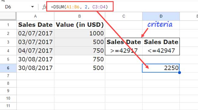
Here are the criteria hardcoded version of the formula:
Curly Braces:
=DSUM(A1:B6, 2, {{"Sales Date"; ">="&DATE(2017, 7, 1)}, {"Sales Date"; "<="&DATE(2017, 7, 31)}})VSTACK:
=DSUM(A1:B6, 2, HSTACK(VSTACK("Sales Date", ">="&DATE(2017, 7, 1)) ,VSTACK("Sales Date", "<="&DATE(2017, 7, 31))))Before concluding, see one more example of using date difference or date range as criteria in DSUM in Google Sheets.
Date with Comparison Operator and Text Conditions in Database Function
The DSUM example below utilizes multiple date conditions as well as text conditions. I’ll resort to screenshots to show you the criteria part, as we won’t hardcode them. Hardcoding these types of multiple criteria in DSUM will make the formula complex.
See the criteria fields at the top (A2:D4), where you can observe that I’ve used multiple dates as well as text conditions.
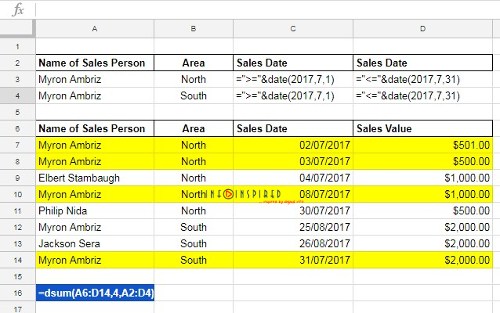
I’ve used the View > Show > Formulae menu option to display the formula entered in cell A16, as well as the date difference criteria in C3:D4.
In the actual case, the date criteria in C3:D4 will look different. Please refer to the image below.
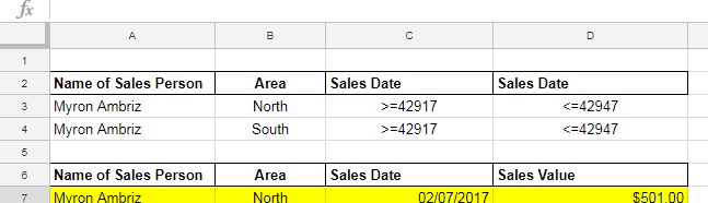
Hope you can understand!
Resources
DSUM is highly useful for conditionally summing values from a table-like range. Date or date difference criteria are crucial components of this conditional sum, as discussed in detail above. The following tutorials may help you further advance in DSUM.