


")


Creating a month-wise summary report in Google Sheets is not a difficult task. A few good options are available, such as the Pivot Table, the SUMIF function, and the QUERY function.
In Excel, there are plenty of options. We can use menu commands such as Data > Subtotal and Insert > Pivot Table and use functions such as SUMIF, SUMIFS, etc.
In Google Sheets also, you can adopt all these methods except the Subtotal. In addition, we can use the QUERY function, the most versatile function in Google Sheets.
So, in this tutorial, let’s learn how to create a month-wise summary report in Google Sheets with the help of the QUERY function.
How to Create a Month Wise Summary Report in Google Sheets
Sample Data:
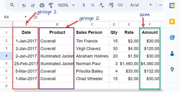
What are we going to do with this data?
We will prepare a month-wise summary of each product by grouping the date and product column.
Please follow the step-by-step instructions below.
Step 1: Group by Month
Syntax: QUERY(data, query, [headers])
The following QUERY formula can be used to group a date column by month and sum another column in Google Sheets:
=QUERY(A1:F,"SELECT MONTH(A), SUM(F) GROUP BY MONTH(A)",1)The formula takes three arguments:
- The range of data to be queried, which is
A1:Fin this case. - The query statement, which is
SELECT MONTH(A), SUM(F) GROUP BY MONTH(A)within double quotation marks in this case. - The number of header rows, which is
1in this case.
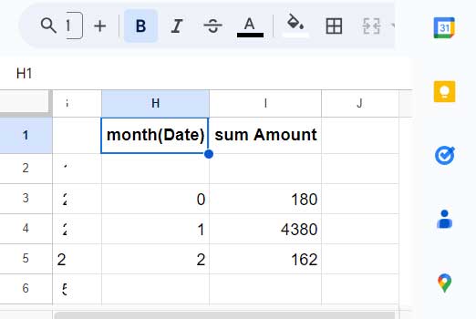
The query statement selects the months of the dates in column A and sums the values in column F, grouping the results by month.
The above month-wise summary result in Google Sheets has three issues:
- The month numbers are ‘incorrect’ because the MONTH scalar function in QUERY returns month numbers as zero-based integers. January is shown as 0, February as 1, and so on.
- There are blank rows in the result.
- The labels are not tidy.
Let’s fix these issues first.
The following formula will adjust month numbers.
=QUERY(A1:F,"SELECT MONTH(A)+1, SUM(F) GROUP BY MONTH(A)+1",1)This one will remove blank rows.
=QUERY(A1:F,"SELECT MONTH(A)+1, SUM(F) WHERE A IS NOT NULL GROUP BY MONTH(A)+1",1)Now what is left is making the labels tidy. We can use the LABEL clause for that.
=QUERY(A1:F,"SELECT MONTH(A)+1, SUM(F) WHERE A IS NOT NULL GROUP BY MONTH(A)+1 LABEL MONTH(A)+1 'MONTH', SUM(F)'TOTAL'",1)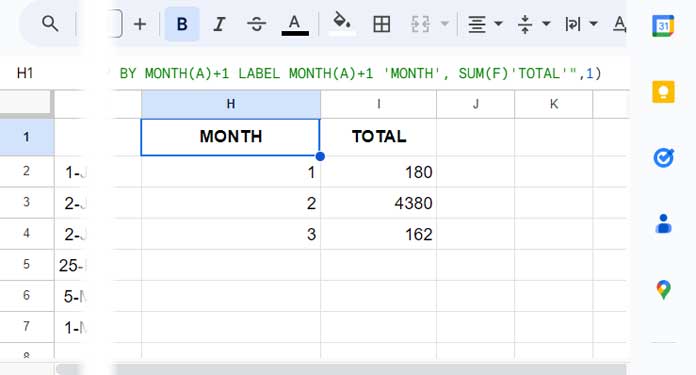
You May Like: What is the Correct Clause Order in Google Sheets Query?
We have created a basic month-wise summary report in Google Sheets. It contains just two columns: A month column and a total column.
Step 2: Group by Month and Product
To group by Product, include it in both the SELECT and GROUP BY clauses. Here is the final formula:
=QUERY(A1:F,"SELECT MONTH(A)+1,B, SUM(F) WHERE A IS NOT NULL GROUP BY MONTH(A)+1,B LABEL MONTH(A)+1 'MONTH', SUM(F)'TOTAL'",1)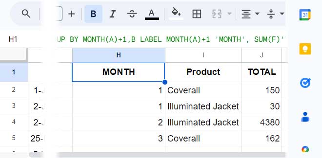
We have created a month-wise summary report using QUERY in Google Sheets.
COUNT, AVERAGE, MIN, and MAX in Month Wise Summary in Google Sheets
When you create a month-wise summary report using the QUERY function, you can use aggregation functions other than the SUM function.
For example, you can use the QUERY AVG, COUNT, MAX, and MIN aggregation functions to calculate the average, count, maximum, and minimum values in a group of data.
For example, to create a monthly average sales summary of products, you could use the following formula:
=QUERY(A1:F,"SELECT MONTH(A)+1,B, AVG(F) WHERE A IS NOT NULL GROUP BY MONTH(A)+1,B LABEL MONTH(A)+1 'MONTH', AVG(F)'TOTAL'",1)Conclusion
When replacing QUERY data with imported data, such as an IMPORTRANGE formula, you must replace column identifiers in the query statement with column numbers.
You would use Col1 to represent the first column in the imported data, Col2 to the second column, and so forth.
Here is an example formula:
=QUERY(IMPORTRANGE("URL","Sheet1!A1:F"),"SELECT MONTH(Col1)+1,Col2, AVG(Col6) WHERE Col1 IS NOT NULL GROUP BY MONTH(Col1)+1,Col2 LABEL MONTH(Col1)+1 'MONTH', AVG(Col6)'TOTAL'",1)We have created a month-wise summary report that uses month numbers for grouping. If you would like to use month names instead, you can use the EOMONTH function in the QUERY data.
You may find these tutorials useful:
Hi Prashant,
Thank you for your help. I am still facing a bit of a mystery with my query. When I add filtering on dates, everything goes wrong.
Here is my query with date filtering:
"Select Col1, sum(Col2) whereCol3 matches true
and Col1 < date '"&text(eomonth(B5, 0),"yyyy-mm-dd")&"'
group by Col1
label sum(Col2) ''")
where B5 contains 2023-07-12
I am expecting the result to be the following:
2023-06-30 -1000
Instead, it gives me an error saying the request ended with no results.
Any idea how to solve this?
Thank you,
Hi Bastien,
Your formula seems correct to me. Can you share an example sheet with me? If so, please leave the URL in the comments below.
Best,
Hi Prashanth,
Here is a testing sheet.
[URL removed by admin]
The tab named “test” contains my trials. The problem occurs in cell G1.
Please take a look and let me know if you have any questions.
I’ve inserted my solution in cell D1 of the sheet named “pkv”. I hope this helps.
Prashant,
Thanks for your post. It has helped me summarise my data by month. There is a slight challenge. If the data ranges from May 2018 to Jul 2019 then it does not show the months as 13, 14, 15, etc. It combines the data for May 2018 with May 2019. Can you please provide a solution for this?
Hi,
There is a different approach using month and year in the summary. I have already included the link to that topic in this tutorial.
Best,