I am confident that you will find creating an Ageing Analysis report using Google Sheets formulas to be a tremendous time-saver.

Upon completing this age analysis spreadsheet, you’ll observe that your data automatically shifts among columns based on ageing.

This means that once you’ve generated the Ageing Analysis report, you can leave it untouched. The formulas in your sheet will automatically adjust the amounts in age-wise columns, eliminating the need for manual cutting and pasting.

While the best method for creating an Age Analysis report in a spreadsheet is by using a Pivot Table, you can also craft a custom Ageing Analysis report using Google Sheets’ IF or IFS logical functions, which is relatively straightforward.

In this post, you’ll learn how to create an Accounts Receivable Ageing Analysis report in Google Sheets, all accomplished through formulas. By the way, you can similarly create an Accounts Payable Age Analysis.

Let’s now proceed with the steps to create an Ageing Analysis report using Google Sheets formulas.

Ageing Analysis Report Using Google Sheets Formula

This is a straightforward tutorial to follow. I’ll share my example sheet below, and you can preview and make a copy of it by clicking the button provided.

Example Sheet

Please proceed with this tutorial to create a custom Ageing Analysis report in Google Sheets.

Data Formatting for Age Analysis

Below is the format of the Ageing Analysis report that we are going to prepare in Google Sheets using formulas.

In other words, our completed accounts receivable age analysis report will resemble the format below.

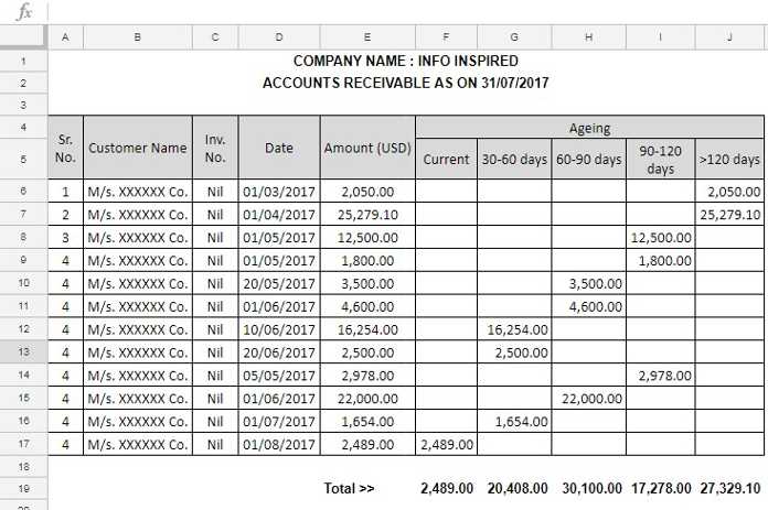
As a side note, please don’t consider the above data seriously. It’s just sample data, so treat it accordingly. Feel free to use your data for the experiment.

Steps for Inserting IF Logical Array Formulas

Prepare the above format and fill in the data, except in the highlighted cells as shown in the image below.

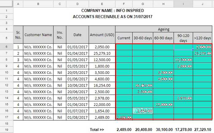
In the highlighted cells, we are going to apply a few IF formulas, which will automatically adjust the value columns based on ageing.

You only need to input the formulas in the first row (here, row #6).

Must Read: Combined Use of IF, AND, OR Logical Test in Google Sheets.

Insert the following formulas in the respective cells. That’s all you need to do to complete your Accounts Receivable Report.

Enter the following formula in cell F6. All are Array Formulas, making them auto-expanding to the rows down.

=ArrayFormula(IF(TODAY()-D6:D17<30, E6:E17, ""))

Here is the formula for cell G6.

=ArrayFormula(IF((TODAY()-D6:D17>29)*(TODAY()-D6:D17<60)=1, E6:E17, ""))

Enter this formula in cell H6.

=ArrayFormula(IF((TODAY()-D6:D17>59)*(TODAY()-D6:D17<90)=1, E6:E17, ""))

In cell I6.

=ArrayFormula(IF((TODAY()-D6:D17>89)*(TODAY()-D6:D17<121)=1, E6:E17, ""))

The final formula is to be entered in cell J6.

=ArrayFormula(IF(TODAY()-D6:D17>120, E6:E17, ""))

You have now completed the Ageing Analysis Report. It’s that easy!

Please modify the dates in the “Date” column, located in column D, to observe how the invoice values shift across the columns based on ageing.

Feel free to add or insert as many rows as needed by adjusting the range reference in the formulas. However, exercise caution when adding new columns to the right or between Columns F and J, as it may lead to unintended results.

If you are unfamiliar with any of the functions used, you can refer to my Functions Guide for clarification.

Related Reading:

1. Age Analysis Using QUERY Function in Google Sheets.
2. Create an Age Analysis Report Using Google Sheet Pivot Table.
3. Drill Down Detail in Pivot Table in Google Sheets [Date Grouping].