


")


This post has step-by-step instructions to help you quickly create an age analysis report using the Pivot table in Google Sheets.
In our example, we will use the Pivot table to place outstanding customer invoice amounts under different categories of the date range of 30 days each in columns.
It will help you find how long a bill has gone unpaid and follow up accordingly.
I posted a tutorial on creating an aging analysis report using Google sheet formulas in the recent past. That report is highly customizable.
Age analysis report using Pivot table is easy to create in Google Sheets, but customization is limited.
Preparation of Sample Data for Age Analysis Report
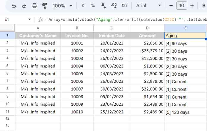
Our sample data contains the customer name, invoice number, invoice date, and invoice amount columns.
In addition to that, we require one helper column to create an age analysis report using the Pivot table in Google Sheets.
Let us go to the steps. I will explain all the details below.
Sample Data (Source Data):

The above is the data format you require first to create a Pivot table aging analysis report.
It contains the outstanding invoices of only one customer because we are creating a simple aging analysis report using the Pivot table in Google Sheets.
Once learned, you can add more customer invoices to the bottom of the table (I’ll show you the screenshot of the finished report with more than one customer at the end of this tutorial).
Empty column E because that acts as our helper column. Then insert the following array formula in cell E1.
=vstack("Ageing",byrow(C2:C,lambda(r,iferror(let(dueby,if(datevalue(r),datedif(r,today(),"D"),),if(and(dueby>=0,dueby<=30),"[1] Current",if(and(dueby>30,dueby<=60),"[2] 30 days",if(and(dueby>60,dueby<=90),"[3] 60 days",if(and(dueby>90,dueby<=120),"[4] 90 days",if(dueby>120,"[5] 120 days")))))),))))It is the only formula that requires to create our report.
What does it do?
It returns the aging of invoices in a custom text format in column E.
| Age | Custom Text |
| 0 to 30 | [1] Current |
| 31 to 60 | [2] 30 days |
| 61 to 90 | [3] 60 days |
| 91 to 120 | [4] 90 days |
| 120 above | [5] 120 days |
Feel free to modify the custom text in the formula. But keep the numbers in square brackets as they are a must for auto-sorting columns by aging.
Now we are ready with the data format. Let’s create a Pivot table Ageing Report using this data in a flash.
Steps to Create Age Analysis Report Using Google Sheets Pivot Table
Steps:
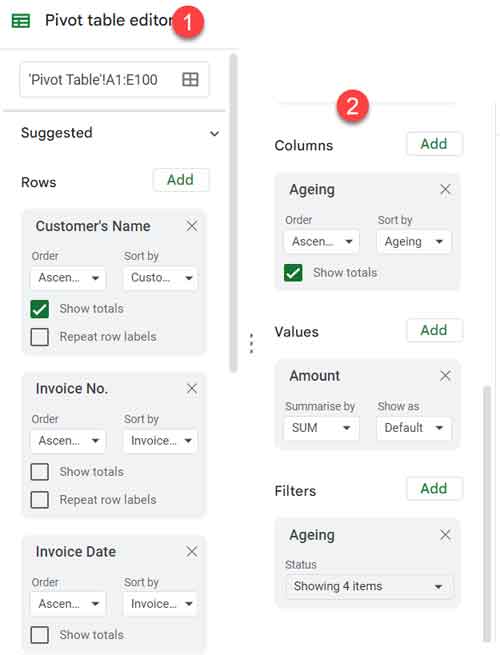
- Select the data range A1:E11. Select more rows if you expect future data entries below row # 11. I mean, instead of A1:E11, select A1:E100.
- Go to the Insert Menu > Pivot table.
- Choose “Existing Sheet” or “New Sheet” based on where you want to insert your age analysis Pivot table report. I’m selecting “Existing Sheet,” cell F1.
- Click the “Create” button.
- Drag and drop “Customer’s Name,” “Invoice No.,” and “Invoice Date” under the “Rows” field.
- Drag and drop “Ageing” under the “Columns” field.
- Uncheck “Show totals” against “Invoice Date” and “Invoice No.”
- Drag and drop “Amount” under the “Values” field.
- Add “Ageing” under “Filter” and uncheck “Blanks.”
Note:- When you add future data to your source data, you should check back the filter (point # 9 above) and re-apply it.
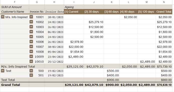
That’s all you should do. Your age analysis report using the Pivot table is ready now (please scroll down to see the image).
Customization of Age Analysis Report in Google Sheets
There are two main customization options available.
One is the Format menu Theme. Switch between different themes and set a suitable one.
Please remember that the theme changes affect an entire file.
The second customization is only for the Pivot table report. To do that, select the pivot table range and apply the Format menu “Alternating colors.” To edit, go to Format > Conditional formatting.
As a side note, if you have multiple customers in your report, select “Show details” against “Invoice No.” in the pivot editor, as mentioned in point#7 above.
That way, you can get subtotal in your Pivot table report in Google Sheets.
See the finished aging analysis report created using the Pivot table below (I’ve added one more customer to show you how the subtotal works).
Advanced Pivot Table Tutorials:
You can simplify your formula:
=IF(E2<30,"1. CURRENT",IF(E2<60,"2. 30-60 DAYS",IF(E2<90,"3. 60-90 DAYS",IF(E229,E2<60)(and others like it) because the earlier tests would include those under 30 days.Plus, don't most aging reports do <30, 31-60, 61-90, 91-120, and 121+ so those at 30, 60, 90, and 120 days are explicitly in a single group? Thus:
=IF(E2<30,"1. CURRENT",IF(E2<60,"2. 31-60 DAYS",IF(E2<90,"3. 61-90 DAYS",IF(E2<119,"4. 91-120 DAYS","5. 121 DAYS & ABOVE"))))