Unlike many other Google Sheets functions it’s not easy to explain GoogleFinance function in a single post. So you can learn this function partly here. This time you can learn how to use GoogleFinance to Convert Currency in Google Sheets. In addition to this, you can learn how to get the list of auto-updating latest currency exchange rates in Google Sheets.

GoogleFinance Function in Google Sheets

GoogleFinance is a very useful function in Google Sheets for those who are dealing with stock markets as it can import current as well as historical security information into Google Sheets. Further, it’s possible in Google Sheets to get the current and historical currency exchange rates using this function. Google fetches these pieces of information from Google Finance.

Syntax of GoogleFinance Function:

GOOGLEFINANCE(ticker, [attribute], [start_date], [end_date|num_days], [interval])

In this Spreadsheet tutorial, I am only going to touch the Currency Exchange part of GoogleFinance function. Let me explain how to convert Currency in Google Sheets.

Get Latest Currency Exchange Rates of All Currencies in Google Sheets

If your business is located in different countries like US, UK, Canada, Japan, France, China, India like any other countries, it’s a must for you to know the current currency exchange rates.

You should know how much quantity of one currency is required ( for example US Dollar) to buy or sell one unit of the other currency (for example Indian Rupee).

In other words, what is the price of the currency of your country in terms of the currency in the country where your business is? So you can make or receive the payments accordingly. Further, you can track overseas cash flow in your own currency. With GoogleFinance function it’s possible to get the current as well as historical currency exchange rates in Google Sheets.

What is Historical Currency Exchange Rates?

The GoogleFinance Function has the option to import currency exchange rates of a specific period, or day in the past. Such data is called historic Currency Exchange Rates.

How to Convert Currency in Google Sheets

Example 1:

Formula:

=GoogleFinance("CURRENCY:USDINR")

Result: 63.575

This formula returns the exchange rate of USD with INR. That means 1 USD = 63.575 INR. The above 63.575 is the exchange rate of USD to INR at the time of writing this post.

If you apply this formula to your sheet you may get a different rate as the exchange rate is auto-updating on Google Sheets. That means GoogleFinance is a Volatile function like the Date and Time functions.

In the above formula “USD” is the currency code of US Dollar and INR is the currency code of Indian Rupee. So one thing is sure. What is that?

You must know the currency codes of all currencies to use GoogleFinance function in Google Sheets. You can find that tips below.

In the above example, you can simply change the “USDINR” (from US Dollar to Indian Rupee) to any other currency.

Import ISO 4217 Currency Codes in Google Sheets

A very simple formula can import all the world currency in Google Sheets along with their ISO 4217 Currency Codes.

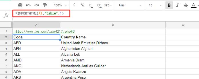
This www.xe.com page contains the list. We can use IMPORTHTML as below in Google Sheet to import the currency and currency codes to Google Sheets.

See the web page link in A1 and the formula in A2. This formula can import all the Currency Codes in Google sheets along with the associated country names. Please note that this screenshot only contains part of the imported data.

In the above screenshot, column C is left blank. There you can get the current currency exchange rates using the GoogleFinace formula.

That means with the help of two formulas (one IMPORTHTML and the other GOOGLEFINANCE), you can get the current currency exchange rates of all the currencies in the world in Google Sheets. See that details under the below title.

Create Currency Exchange Rates Table in Google Sheets Using GoogleFinace Function (1 USD Rates Table)

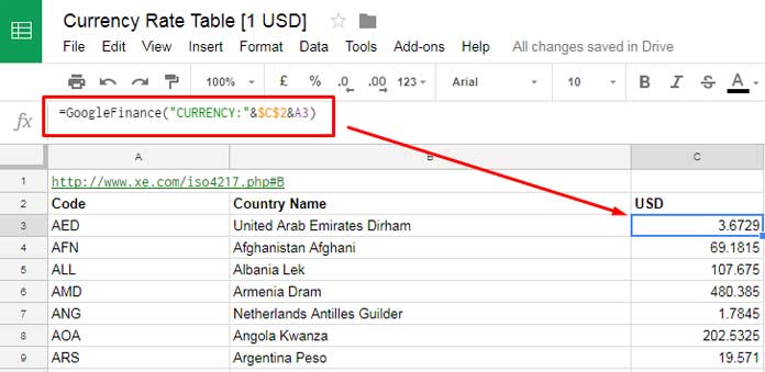
In the above example, we have imported all the currency and currency codes into Google Sheets. As already told, you can see column the C, left as blank. I’m going to apply GoogleFinance formula there to get the current currency exchanges rates (1 US Dollar rate or you can say 1 US Dollar equal to how much other currencies) of all the currencies in the world.

In cell C2 the text entered is “USD”. You can change this to INR to get 1 INR Rates.

The below is the formula in C3. You need to copy and paste this formula to down to get the exchange rates of all currencies.

Formula:

=GoogleFinance("CURRENCY:"&$C$2&A3)

Actually, you can read the formula in C3 as below that without cell references.

=GoogleFinance("CURRENCY:USDAED")

How to Get Currency Exchange Rate of a Specific Date in Google Sheets

This section handles the historical currency exchange rates. Convert Currency in Google Sheets, but of a specific date or dates.

Currency Exchange Rate of a Specific Date

When you want to get the currency exchange rate of any currency in a specific date, the formula would be as below.

Formula: =GOOGLEFINANCE("CURRENCY:USDEUR", "price", DATE(2017,9,1))

This formula returns the exchange rate of USD with EUR on 01/09/2017.

Currency Exchange Rates of Specific Dates

When you want to get currency exchange rates for a time period, called historical data, the formula would be as below with starting and end date.

=GOOGLEFINANCE("CURRENCY:USDINR", "price", DATE(2017,12,1), DATE(2017,12,31), "DAILY")

The above formula returns the currency exchange rates of USD with INR for the month of December.

How to Automate Currency Conversion and SUM

When you have the source of income from different countries, and in different currencies, you can automate the conversion of all that currencies to your currency and sum.

Below you can find one example.

In column D, I’ve added the formula separately for your reference.

In the above example, you can see that currency from USD, ILS and AUD are converted to INR and then summed.

For example, in C2 I have taken the exchange rate from USD to INR and multiplied it with the value in B2.

How to Remove Header Label in GoogleFinance Historical Data

When you import historical exchange rates of a currency of a specific period, the GoogleFinance function may return the output as below with column label.

You can see the column label “Date” and “Close”. How to remove these column labels in GoogleFinance in Google Sheets?

=query(GOOGLEFINANCE("CURRENCY:USDEUR", "price", DATE(2017,12,20)),"SELECT Col1, Col2 label Col1 '', Col2 ''")

A Query as above can sort out this issue. That’s all. Hope you have learned how to Convert Currency in Google Sheets Using GoogleFinance Function.