With the assistance of lookup functions, we can compare two columns for both matching and mismatching values in Google Sheets.

I prefer using the XMATCH function for this task, as it is one of the most modern lookup functions in Google Sheets.

Comparing columns for matches or mismatches is a valuable technique that proves beneficial in real-life scenarios. For instance, you can match the requirements of vehicle parts in one column with the stock in another column.

Comparing Two Columns for Matching Values

This is not a quantity-wise comparison; instead, it’s an item-wise comparison. For the test, we have the stock of vehicle parts in Column A (names) and requirements (names) in Column B.

Let’s compare these two columns, A and B, with the data range being A2:A and B2:B, considering that A1 and B1 contain field labels.

Initially, we will compare Column B (required parts) with A (stock).

Find Matching Values in Column B from Column A

The following formula will return tick marks against the required items if they are found in the stock.

=ArrayFormula(IF(IFNA(XMATCH(B2:B, A2:A)), "x", ))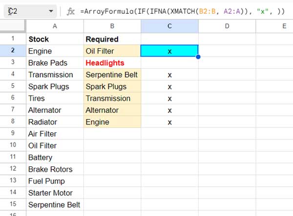

You can enter this formula in cell C2. Before you input this formula, please ensure two things:

1. C2:C must be blank: Select C2:C and hit the delete key to remove everything in this range.
2. Enter the formula where the row of the comparing column ranges begins: In our example, the ranges are A2:A and B2:B, with row #2 being the starting row. Therefore, it’s suggested to insert the formula in C2.

Anatomy of the Formula:

It’s an XMATCH array formula where B2:B is the search key, and A2:A is the lookup range.

The formula searches the values in B2:B in A2:A and returns relative positions of matching values. If there is no match, the formula returns #N/A, and the IFNA wrapper removes those errors. What’s left are the relative positions of matching items.

For readability, we have used an IF logical test to convert those relative positions to “x.” An “x” indicates that it found matches in column A. If you prefer, you can replace relative positions with a green tick mark. For that, replace “x” in the formula with CHAR(9989).

This is an example of comparing two columns for matching values in Google Sheets. Let’s move on to another example.

Find Matching Values in Column A from Column B

Here is a different scenario for comparing two columns. Suppose you want to identify the items in the stock that are sought. In other words, find matching values in Column A from Column B.

For that, we can use the XMATCH formula with minor changes. In XMATCH, replace the search key with A2:A and the lookup range with B2:B.

Formula:

=ArrayFormula(IF(IFNA(XMATCH(A2:A, B2:B)), "x", ))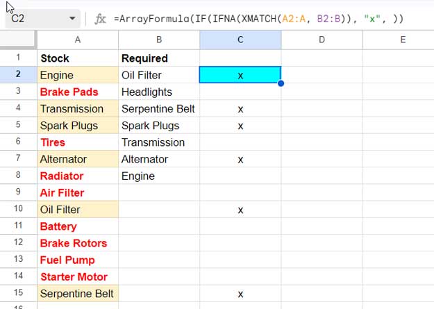

The formula returns a checkmark next to the stock items that are sought.

With this example, we conclude the comparison of two columns for matching values. Let’s now proceed to compare two columns for mismatching values.

Compare Two Columns for Mismatching Values

Comparing two columns for mismatching values is slightly different from comparing matching values. For example, you can use it to mark the items that are not available in the stock or mark the non-required items in the stock. The latter is less common in use, but I will include that too.

Formula to Find Mismatching Values in Column B from Column A:

=ArrayFormula(IF(B2:B="", ,IFNA(IF(XMATCH(B2:B, A2:A),), "x")))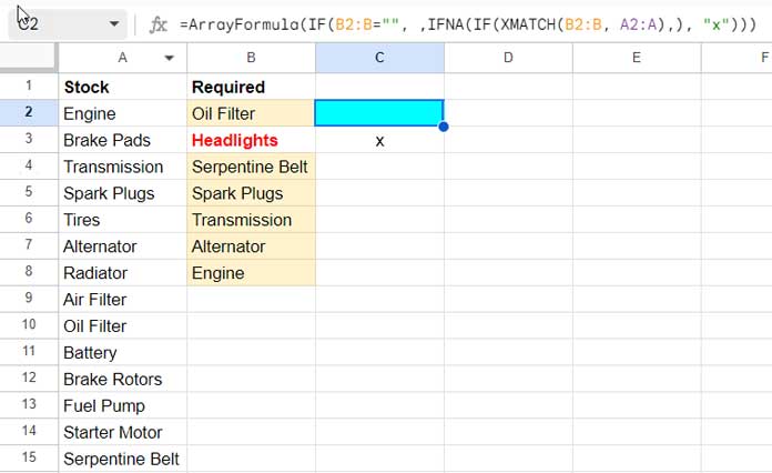

This formula will return “x” marks in rows next to the required parts where they are not available in the stock.

Formula to Find Mismatching Values in Column A from Column B:

=ArrayFormula(IF(A2:A="", ,IFNA(IF(XMATCH(A2:A, B2:B),), "x")))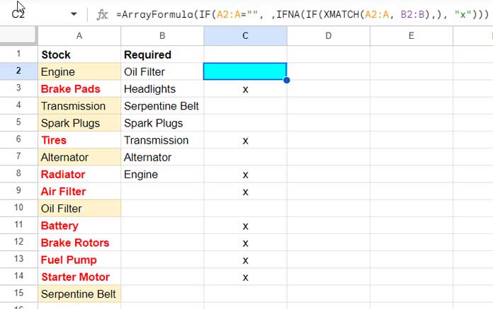

This formula will return “x” marks next to the stock items that are not found in the required list. It’s not as commonly used.

Anatomy of the Formula:

Let me explain these two formulas in comparison to the formulas that we used for comparing two columns for matching values.

• In the earlier formulas, we used IFNA to remove #N/A errors. Here, instead, we have used it to convert #N/A to “x”.
• In the earlier formulas, the IF converted relative positions to “x”. Here, instead, it removes relative positions.
• In addition to the above two changes, we have employed another IF logical test, i.e., IF(B2:B="", or IF(A2:A="", to return blank in rows where the search keys (column to compare) are blank. This will prevent the formulas from leaving check marks in empty rows.

Resources

• Formula to Find Partial Match in Two Columns in Google Sheets
• Match Two Columns that Contain Values Not in Any Order Using Rege
• Google Sheets: Compare Two Lists and Extract the Differences
• Highlight Matches or Differences in Two Lists in Google Sheets