


")


Comparing SUMIFS, SUMPRODUCT, and DSUM matters in Google Sheets because they calculate sums based on conditions in a range.
Among these three, SUMIFS and DSUM are two dedicated functions for conditional sums. While SUMPRODUCT can be utilized for this purpose, it is primarily designed for returning the sum of products.
I have already created two tutorials that will provide you with insights into the distinctions between these functions:
- Difference Between SUMIFS and DSUM in Google Sheets
- Differences Between SUMIFS and SUMPRODUCT Functions in Google Sheets
In this tutorial, we will use these functions to address identical issues or challenges. This approach will help you understand their differences and determine which one is more convenient for your specific needs.
In addition, I’ll highlight my recommended function for the specific purpose mentioned in the examples below.
Sample Data (Range A1:D):
| Name | Category | Date | Amount |
| John | Category A | 15/01/2022 | 100 |
| Alice | Category B | 20/02/2022 | 150 |
| Bob | Category A | 15/01/2022 | 120 |
| Mary | Category C | 10/03/2022 | 80 |
| David | Category B | 20/02/2022 | 200 |
| Emma | Category C | 10/03/2022 | 90 |
| John | Category C | 10/03/2022 | 50 |
This table includes names, categories, dates, and amounts. You can utilize the SUMIFS, SUMPRODUCT, and DSUM functions to calculate the total amount based on specific conditions.
SUMIFS, SUMPRODUCT, and DSUM: Criteria as Cell References
Single Criterion
How do we total column D for dates in column C that are greater than or equal to 1 February 2022?
Using DSUM:
DSUM is a Database category function (Insert > Function > Database > DSUM) in Google Sheets that returns the sum of values from a table-like range.
We have a table-like range (structured data) above (data arranged under field labels in columns and no merging of cells is done).
Syntax:
DSUM(database, field, criteria)Formula:
=DSUM(A1:D, "Amount", F2:F3)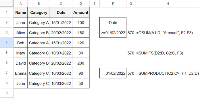
Where:
database: A1:Dfield: “Amount” – this is the field to sum. You can also use the field index number, which is 4.criteria: F2:F3 – F2 contains the label “Date,” and F3 contains the criterion formula, which is=JOIN("", ">=", DATE(2022, 2, 1)).
The DATE function is in the syntax DATE(year, month, day).
Using SUMIFS:
SUMIFS is a Maths category function (Insert > Function > Maths > SUMIFS) in Google Sheets that returns the sum of a range based on multiple criteria.
Syntax:
SUMIFS(sum_range, criteria_range1, criterion1, [criteria_range2, …], [criterion2, …])Formula: ✅
=SUMIFS(D2:D, C2:C, F3)Where:
sum_range: D2:Dcriteria_range1: C2:Ccriterion1: F3 – F3 contains the formula=JOIN("", ">=", DATE(2022, 2, 1)). Please refer to the image above.
Using SUMPRODUCT:
SUMPRODUCT is an Array category function (Insert > Function > Array > SUMPRODUCT) in Google Sheets that is used to return the sum of products of elements in two arrays.
Syntax:
SUMPRODUCT(array1, [array2, …])Formula:
=SUMPRODUCT(C2:C>=F7, D2:D)Where:
array1: C2:C>=F7 – F7 contains the date 1 February 2022. This part returns TRUE (matches) or FALSE (mismatches).array2: D2:D
The array1 contains TRUE or FALSE values where TRUE is equal to 1, and FALSE is equal to 0.
The formula multiplies array1 and array2 and returns the sum.
The above are the comparisons of SUMIFS, SUMPRODUCT, and DSUM using a criterion in Google Sheets.
Multiple Criteria
This time we have the following criteria in the range F2:G4 where F2:G2 contains the field labels Name and Category, respectively.
| Name | Category |
| Mary | Category C |
| Emma |
This table-like criteria arrangement is specifically meant for DSUM. The other two functions do not require this arrangement, as you will see in the examples below.
The purpose is to sum the Amount column filtering Category C in column B and names Mary and Emma in column A.
DSUM: ✅
=DSUM(A1:D, "Amount", F2:G4)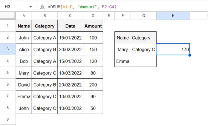
SUMIFS:
=ArrayFormula(SUMIFS(D2:D, B2:B, G3, (A2:A=F3)+(A2:A=F4), 1))The ArrayFormula is required since we calculate (A2:A=F3)+(A2:A=F4) which returns 1 if it matches either F3 or F4, else 0.
SUMPRODUCT:
=SUMPRODUCT((B2:B=G3)*((A2:A=F3)+(A2:A=F4)), D2:D)SUMPRODUCT doesn’t require the ArrayFormula function, as it is already an array function.
SUMIFS, SUMPRODUCT, and DSUM: Hardcoded Criteria
Sometimes, we use criteria within the formula called hardcoded. I advise against using DSUM with hardcoded criteria for the conditional sum as it is very complex.
For comparison purposes, I’ll include all these three functions, SUMIFS, SUMPRODUCT, and DSUM, with hardcoded criteria.
Single Criterion:
To sum column D for column C is greater than or equal to 1 February 2022, use the below formulas.
=DSUM(A1:D, "Amount", VSTACK("Date", JOIN("", ">=", DATE(2022, 2, 1))))
=SUMIFS(D2:D, C2:C, JOIN("", ">=", DATE(2022, 2, 1))) // ✅
=SUMPRODUCT(C2:C>=DATE(2022, 2, 1), D2:D)
Multiple Criteria:
To sum column D for column A is equal to Mary or Emma, and column B is equal to Category C
=DSUM(A1:D, "Amount", IFNA(HSTACK(VSTACK("Name", "Mary", "Emma"), VSTACK("Category", "Category C"))))
=ArrayFormula(SUMIFS(D2:D, B2:B, "Category C", (A2:A="Mary")+(A2:A="Emma"), 1))
=SUMPRODUCT((B2:B="Category C")*((A2:A="Mary")+(A2:A="Emma")), D2:D) // ✅
In DSUM, we employed VSTACK and HSTACK functions to craft a table-like array for criteria. Proficiency in creating such table structures is essential for this process.
I hope these formulas help you understand the differences between the SUMIFS, SUMPRODUCT, and DSUM functions in Google Sheets.
Resources
In a nutshell, when you compare SUMIFS, SUMPRODUCT, and DSUM in Google Sheets, you’re getting to know how each one helps you add up data under certain conditions. This understanding gives you a bunch of useful tools to work with your data more effectively. If you’re interested, here are some extra resources related to these functions.
- How to Use Date Difference as Criteria in DSUM in Google Sheets
- How to Use Date Differences as Criteria in SUMPRODUCT in Google Sheets
- Using Different Criteria in the SUMIFS Function in Google Sheets
- How to Do a Case-Sensitive DSUM in Google Sheets
- How to Do a Case Sensitive Sumproduct in Google Sheets
- REGEXMATCH in SUMIFS and Multiple Criteria Columns in Google Sheets
- AND, OR in Multiple Criteria DSUM in Google Sheets (Within Formula)
- How to Use OR Condition in SUMPRODUCT in Google Sheets
- SUMIFS with OR Condition in Google Sheets
- Google Sheets: How to Use Multiple Sum Columns in DSUM Function
- How to Use SUMIFS to Sum Multiple Columns in Google Sheets