


The CHOOSE function in Google Sheets might not be the most powerful tool for lookups, but it’s simple and easy to learn, making it a useful tool in your spreadsheet toolbox. Don’t overlook its versatility!
Beyond basic lookups, CHOOSE can be used creatively. Think about naming ranges and using CHOOSE to switch between them in other formulas, crafting dynamic strings that adapt to your data, or generating a smart chip that displays a dynamic star rating. You can even pick a random value, dynamically select functions in a QUERY, and much more!
Even though other Google Sheets functions like IF, IFS, SWITCH, OFFSET, INDEX, MATCH, CHOOSECOLS, and CHOOSEROWS provide more flexibility, the simplicity of CHOOSE is still an advantage. It’s often the most straightforward choice for beginners and those who prefer a clear, simple approach.
Before exploring the various applications of CHOOSE, let’s first understand its syntax and arguments.
CHOOSE Function: Syntax, Arguments, and Basic Examples
Syntax:
CHOOSE(index, choice1, [choice2, …])Arguments:
index: A number between 1 and 29 (both inclusive) or a cell reference containing one of these numbers. If multiple indices are preferred, include the ARRAYFORMULA function.choice1, [choice2,…]: Up to 29 individual values or cell references representing the choices to select from. These choices must be explicitly listed in the formula and cannot be array/range references.- For instance, if the index is 1, the first choice is returned; if the index is 5, the fifth choice is returned, and if the index is 29, the twenty-ninth choice is returned.
choice2,…: Optional.
Basic Examples
I’ve included some of the best examples to help you understand the real-life applications of the CHOOSE lookup function in Google Sheets.
Before we delve into those, let’s explore two basic examples:
=CHOOSE(2, "A", "B", "C")- Returns: “B”
- Explanation: The index number is 2, so the formula returns the second choice, which is “B.”
To return choices 1 and 3, specify the indices as an array using curly braces {1, 3} and wrap the formula with the ARRAYFORMULA function.
Example:
=ArrayFormula(CHOOSE({1, 3}, "A", "B", "C"))In both examples, you can use cell references instead of indices, such as A1 or A1:A2.
These are two fundamental examples showcasing the use of the CHOOSE function in Google Sheets.
Utilizing the CHOOSE Function to Create Dynamic Ranges for Referencing in Other Functions
In this example, we will explore how to select two different arrays within the SUM function dynamically.
Here is the sample data located in cells A1:C5 in a Google Sheets file:
| Subject | Isabella | Ben |
| English | 89 | 94 |
| Maths | 75 | 78 |
| Physics | 92 | 86 |
| Chemistry | 56 | 60 |
Column A contains subject names, and columns B and C contain the marks of the students Isabella and Ben, respectively.
To set up named ranges, select B2:B5 (Isabella’s marks), click on “Data” > “Named ranges,” name the range “Isabella,” and click “Done.” Then select C2:C5 (Ben’s marks), click “Add range” within the sidebar panel, name it “Ben,” and click “Done.”
Enter 1 (index) in cell E2 and use the following formula in cell F2:
=ArrayFormula(CHOOSE(E2, Isabella, Ben))
This formula will return the marks of Isabella in the range F2:F5. If you enter 2 in E2, the marks of Ben will appear.
You can further enhance this by wrapping the CHOOSE function with SUM to total the marks.
=ArrayFormula(SUM(CHOOSE(E2, Isabella, Ben)))This example showcases how to use the CHOOSE function in Google Sheets to create dynamic ranges within other functions.
Using the CHOOSE Function for Smart Chip-Based 5-Star Rating in Google Sheets
Another fascinating application of the CHOOSE function in Google Sheets is creating a dynamic 5-star rating using the Rating Smart Chip.
To implement this:
- Prepare two blank cells for the test, for example, A1 and B1.
- In A1, enter a number from 0 to 5 (representing the scores for rating).
- Move to B1 and click “Insert” > “Smart chips” > “Rating.”
- In B1 (the same cell where the rating Smart chip is inserted), input the following formula:
=CHOOSE(A1+1, 0, 1, 2, 3, 4, 5)The rating will dynamically adjust based on the score entered in cell A1.
In this formula, A1+1 is used instead of A1 as the rating starts from 0 to 5. The numbers 0 to 5 will be in cell A1, and the function supports indices from 1 to 29.
Note: The use of CHOOSE is not necessary here; the example is provided to illustrate its usage. For more details, refer to this related tutorial: “Rate with Ease: Google Sheets’ New Built-In Rating Feature.“
Nested CHOOSE Functions for Dynamic Text String in Google Sheets
In this example, the goal is to replace the placeholder texts with preferences and contacts. The initial text has two placeholders: [preference] and [contact].
Please [preference] us at [contact]To achieve this, nested CHOOSE functions are used to dynamically create the text string:
="Please "&CHOOSE(A3, "E-mail", "call", "WhatsApp")&" us at "&CHOOSE(A3, "abc@example.com", "987654321", "123456789")Explanation: The sentence structure changes based on the value in A3 – “Please E-mail us at abc@example.com” for 1, “Please call us at 987654321” for 2, and “Please WhatsApp us at 123456789” for 3.
Using CHOOSE with RANDBETWEEN for Basic Random Selection
You can employ the RANDBETWEEN function to generate a random number, which can then be used as the index in the CHOOSE function. This approach facilitates random selection.
=CHOOSE(RANDBETWEEN(1, 3), "Mangosteen","Rambutan","Cranberry")The formula above will randomly return one of the fruit names from the choices. It refreshes with each edit in the sheet, providing a dynamic and random selection.
Similar: How to Pick a Random Name in Google Sheets (Does Not Refresh)
Dynamically Choosing Aggregation Functions in Google Sheets QUERY with CHOOSE
Let’s explore how to dynamically choose aggregation functions (avg(), count(), max(), min(), and sum()) within the QUERY function in Google Sheets.
Suppose you wish to aggregate data in column B dynamically.
=QUERY(B1:B,"Select "&CHOOSE(D2, "avg", "count", "max", "min", "sum")&"(B)")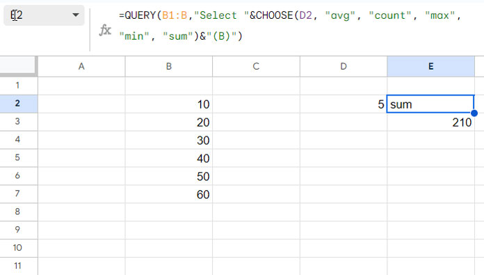
This formula will perform average, count, max, min, or sum operations on column B based on the index number in cell D2.
For instance, if you enter 3 in cell D2, the formula will return the maximum value in column B.
Conclusion
In this exploration, we’ve examined various examples, both basic and advanced, showcasing the application of the CHOOSE function in Google Sheets.
While it’s true that many of these scenarios can be rewritten using other functions with greater flexibility, the CHOOSE function stands out for its intuitiveness and simplicity, making it particularly accessible for beginners.
Despite its limitation of 29 choices, the CHOOSE function remains a valuable tool for straightforward lookups, as demonstrated in the examples above.
Its syntax is clear and uncomplicated, ensuring ease of comprehension even when revisiting formulas in the future.
For those new to spreadsheet functions, the CHOOSE function serves as an excellent starting point. So, don’t hesitate to leverage the CHOOSE function in Google Sheets for your simpler lookup needs.