Case Sensitive Sumproduct is possible in Google Sheets. But not in the way you do it in Excel. I’ll come to that.

I’ve recently written a series of posts related to Case Sensitive Formulas in Google Sheets.

You can use the search field on the top navigation bar with the keyword “Case Sensitive” to fetch links to those posts.

Case Sensitive Sumproduct in Google Sheets

As you know, SUMPRODUCT in Google Sheets is a case In-sensitive function. This function treats “A” and “a” as identical.

So how to make Sumproduct Case Sensitive in Google Sheets?

Here is an example.

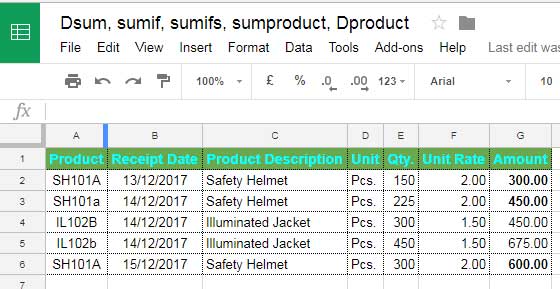
Sample Data:

You may type the above sample data into a plain Google Doc Spreadsheet, keeping the range I have provided.

Now, let’s find the total amount in column G for the Product “SH101A” in column A.

Note:- Please note that the word “Product” above is the field label in cell A1, not the Product in the Sumproduct.

You can see similar products in column A, i.e., “SH101A” and “SH101a”, but both are different w.r.t. case sensitivity.

When you use a standard Sumproduct formula, or you can say case insensitive formula as below, it would return the result 1350.00 as it treats the cells A2, A3, and A6 identical.

Case Insensitive Sumproduct Formula

=SUMPRODUCT((A2:A6="SH101A")*(G2:G6))

Case Sensitive Sumproduct Formula

Now see the Case Sensitive Sumproduct Formula in Google Sheets below, which would return 900.00.

The reason is that it finds the match only in cells A2 and A6.

The array or range A2:A6 in the above case insensitive formula is different in the case-sensitive formula below.

Another change is in the criterion. The text criteria in the first formula, “SH101A”, changed in the second formula to # 1.

=sumproduct((ArrayFormula(- -isnumber(find(A2:A6,"SH101A")))=1)*G2:G6)

In the second formula, I’ve used ArrayFormula, ISNUMBER, and FIND functions to create a virtual array instead of A2:A6. Here is that step by step instructions.

Formula Explanation

The FIND function may not work with an array as below.

=find(A2:A6,"SH101A")

You may want to use the ArrayFormula function with it.

=ArrayFormula(find(A2:A6,"SH101A"))

This formula searches the array A2:A6 for the key “SH101A” and returns # 1 if it finds the exact match. Else it would return #VALUE!.

When you wrap the above ArrayFormula + Find function combined with an ISNUMBER formula, it would modify the output as below.

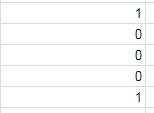
=ArrayFormula(--isnumber(find(A2:A6,"SH101A")))

Result:

This virtual array replaces A2:A6.

Here the numeric value 1 represents the exact match of criteria SH101A, and 0 is a mismatch.

As a result, for this new range, we can use the criteria as numeric value 1, not the text criteria “SH101A”.

In this way, you can convert a Case Insensitive Sumproduct formula to Case Sensitive in Google Sheets.

But in Excel, there is a different approach with the Exact function. Enjoy!

Conclusion

I’ve only given one option above. You can also use regular expressions in this case.

For example, the following formula will return 900, similar to the above formula result.

=ArrayFormula(sumproduct(regexmatch(A2:A6,"^SH101A$")*G2:G6))

Here, the REGEXMATCH (exactly) matches the condition SH101A and returns TRUE (1) or FALSE (0).

So, you can use this formula also for Case Sensitive Sumproduct in Google Sheets.

Advanced Google Docs Sumproduct Function Formulas and Tutorials:

• How to Use Date Difference as Criteria in SUMPRODUCT in Google Sheets.
• Compare Sumifs, Sumproduct, and Dsum with Example in Google Sheets.
• A chart to Learn Text, Date, Numeric Criteria in Sumproduct Function in Google Sheets.
• How to Use OR Condition in SUMPRODUCT in Google Sheets.
• How to Use Wildcards in Sumproduct in Google Sheets.
• Difference Between SUMIFS and SUMPRODUCT in Google Sheets.
• How to Use Sumproduct with Merged Cells In Google Sheets.