


")


I believe Case Sensitive Reverse Vlookup Using Index Match is new to you. Let’s learn that in detail below.
Reverse Vlookup in Google Sheets is Possible with the Index/Match function combo. It is also called backward Vlookup in Google Sheets.
But what about a Case Sensitive Reverse Vlookup in Google Sheets.
Vlookup is the favorite function of all spreadsheets aspirants. But it has a few drawbacks.
The most prominent one among them is reverse Vlookup or backward Vlookup.
That doesn’t mean the reverse vertical lookup is not possible using the function Vlookup.
It’s possible with a simple workaround. That is detailed here – Reverse Vlookup Examples in Google Sheets [Formula Options].
A combination of the Index and Match function can work similarly to Vlookup, and it’s, in some scenarios, better than Vlookup.
Advanced users like to use the Index Match Combination as an alternative to Vlookup.
Here in this tutorial, you can learn two things – Case Sensitive Index Match and Case Sensitive Reverse Vlookup Using Index Match.
So here we begin.
Case Sensitive Index Match (Case Sensitive Vlookup Alternative)
Case-sensitive Vlookup in Google Doc Spreadsheet is possible.
Scroll down to see the second post title under the subtitle, ‘Resources.’
By using Index Match also, you can do a case-sensitive Vlookup. Here are the sample data and formula.
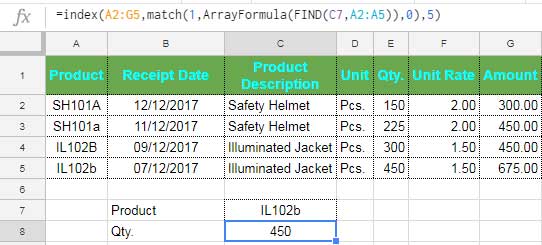
Formula # 1:
=index(A2:G5,match(1,ArrayFormula(FIND(C7,A2:A5)),0),5)Note:- In this ArrayFormula is optional.
Before explaining the above Index Match Case Sensitive formula, see the same Case In-sensitive formula below and its explanation.
Formula # 2:
=INDEX(A2:G5,MATCH(C7,A2:A5,0),5)Index Syntax:
INDEX(REFERENCE, [ROW], [COLUMN])- reference –
A2:G5 - row –
MATCH(C7,A2:A5,0) - column –
5
Here the only confusing part is the “row” argument, right?
We don’t have the number to row offset. Instead, what we have is the search key “IL102b.”
So, I’ve used the Match function to return the offset number.
If you have any further doubt, please check tutorial # 5 in the last part of this post.
We will go straightaway to Case Sensitive Reverse Vlookup after the formula explanation.
Formula Explanation
Scroll up to see the Case Sensitive Index Match formula (formula # 1).
Once again, the confusing part would be the ‘row’ argument in the Index.
Row Offset in Formula # 1: match(1,ArrayFormula(FIND(C7,A2:A5)),0)
Row Offset in Formula # 2: MATCH(C7,A2:A5,0)
Match Syntax:
MATCH(search_key, range, [search_type])In formula # 1, the range within Match is a FIND formula whereas, in formula # 2, it’s A2:A5.
The reason, Find is a case-sensitive function in Google Sheets.
It looks for search key “IL102b” in the range A2:A5 and returns the following array.

Note:- Find is not an array formula. So we should use the ArrayFormula together with it, but optional within Index.
So the search_key in the Match part of formula # 1 is 1, whereas in formula # 2 is C7.
Case Sensitive Reverse Vlookup Using Index Match
One of the main advantages of Index / Match over Vlookup is its flexibility.
Let me explain to you why Index_Match Combo is more flexible than Vlookup.
INDEX(reference, [row], [column])When you check the syntax of the Index, you can understand one thing.
Index returns the content by offsetting the given number of rows and columns.
We manipulate the Row offset using Match. That makes it work similarly to Vlookup.
In the syntax above, reference is the entire data range. Now take a look at the Vlookup Syntax below.
VLOOKUP(search_key, range, index, [is_sorted])The “Reference” in the Index Function is equal to the “range” in the Vlookup. Similarly “Column” is equal to “Index”.
But the “row” in the Index is not the “search_key” in Vlookup.
To act it as the “search_key,” we should use the Match function with “row” in the Index that we have already seen in the above example.
This “row” element of the Index function makes it flexible. How?
In Vlookup, we should directly input the “search_key,” either within the formula or as a cell reference.
In Index, we find the “row” using a search key from a range. This range can be any column in your data set.
But in standard Vlookup, the search key should be from the left-most column.
That’s why Index / Match is flexible, and we can use it for reverse lookup.
Note:
You can use Vlookup too for Reverse Lookup! See this link – Vlookup in Google Sheets – 10 Formula Variations, Tips, and Trick.
Example – Case Sensitive Reverse Vlookup Using Index Match
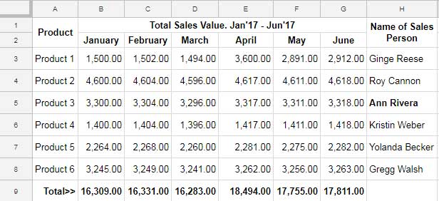
Here I want to find the Sales Value of one Sales Person “Ann Rivera, for January.
The salesperson’s name is in the right-most column, i.e., column H, and the output we require from column B.
So we need to lookup backward in column B (Index # 2). The formula is as follows.
Formula # 3:
=index(A3:H8,match(1,arrayformula(find(H3:H8,"Ann Rivera")),0),2)Result: 3,300.00
The formula is case-sensitive because of the use of Find for search.
If you want to solve the same with Vlookup, use REGEXMATCH with it. Here is the alternative to the above formula # 3.
=vlookup(true,{ArrayFormula(REGEXMATCH(H3:H8,"^"&E13&"$")),A3:G8},3,0)