It’s possible to do a case sensitive DSUM in Google Sheets. But at the same time, I wish to make it clear that you can use Query function to get the same result as Query is case sensitive.

Still, I dedicate this tutorial for those who wish to know how to do a case sensitive DSUM in Google Sheets.

The formula may seem a little complex but nothing to worry, you can catch it.

Here in this tutorial, I am following the same method which I’ve adopted earlier in the case sensitive SUMIF, SUMPRODUCT, and COUNTIF formulas. So let’s begin.

How to Do a Case Sensitive DSUM in Google Sheets

The essence of every tutorial is well-oriented data and especially for DSUM as it’s a database function.

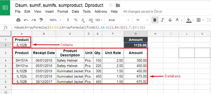
Let me start with a normal case insensitive DSUM formula for the above dataset in A3:G8 and the criterion in A1:A2.

=DSUM(A3:G8,7,A1:A2)

The same case insensitive DSUM formula but the criterion hardcoded.

=DSUM(A3:G8,7,A1:A2)

The criterion here is “IL102B” from the “Product” column.

The DSUM formula would sum column G, i.e. field number 7, wherever the criterion would meet the value “IL102B” in column A, irrespective of its case. That means it would also sum the value for “IL102b”.

Below you can see my case sensitive DSUM formula for the above example in Google Sheets. I’ve tried to compare this with the above normal DSUM formula.

=DSUM(
     ARRAYFORMULA({A3:G3;{ARRAYFORMULA((FIND(A2,A4:A8))),B4:G8}})
     ,7
     ,{A1;1}
)

Formula Explanation

The ARRAYFORMULA part in the above formula actually acts as a virtual ‘database’. Here is the syntax to know the position (order) of the said argument in the formula.

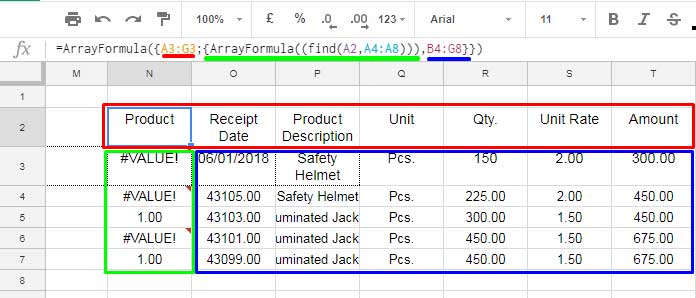
Syntax: DSUM(database, field, criteria)

To explain what this formula does, I’ve just entered the ‘database’ part in cell N2. See the below screenshot where I’ve marked what the combination of formulas does here.

Virtual ‘database’ in Google Sheets

The formula in Cell N2 returns a virtual database in the range N2:T7.

In this (formula) A3:G3 returns the header row (see the values inside the red square) and B4:G8 returns the values except for the values from column A (see the values inside the blue square).

I think only the values in the green-colored square requires little explanation.

As a side note, if you think this’s tough to follow, I’ve shared the link of my Google Spreadsheet at the end of this tutorial. You may please check that.

The green-colored part is a FIND formula in an array form.

The FIND is a case sensitive function which returns 1 if it finds matches and else a “#VALUE!” error. See that part of the formula once again below.

=ARRAYFORMULA((FIND(A2,A4:A8)))

In Cell A2 we have our criteria “IL102B”. This FIND array formula checks this text value in the range A4:A8 and returns an array as above (green colored part in the virtual database screenshot). That’s it.

The Curly Brackets connects all the elements (creates array).

Now we have a virtual database. In this, we can apply a DSUM formula as usual. That’s what our original CASE SENSITIVE DSUM formula does.

You can scroll up and see the original formula just above the title “Formula Explanation”. In that DSUM, instead of criteria range A1:A2, I have used the following criteria.

{A1;1}

This is because, in the first column in our virtual database, the criterion “IL102B” is replaced by the value 1.

So the above criteria would do the job of our original criteria range A1:A2. It simply replaces the value in A2, i.e. “IL102B”, with 1.

If you have any doubt, you can open my Google Sheet below and make a copy of it.

Spend time in your leisure to learn this combination so you can follow this approach to make any case insensitive formula in Google Sheets to case sensitive.

Sample_Sheet_31520

Resources

• Difference Between SUMIFS and DSUM in Google Sheets.
• How to Properly Use Criteria in DSUM in Google Sheets [Chart].
• The Ultimate Guide to Using Criteria in Database Functions in Google Sheets.
• Exact Match in Database Functions in Google Sheets – How-To.
• How to Use Date Difference As Criteria in DSUM in Google Sheets.
• AND, OR in Multiple Criteria DSUM in Google Sheets (Within Formula).
• Google Sheets: How to Use Multiple Sum Columns in the DSUM Function.