


")


Another awesome Google Sheets tutorial! This time, we’ll learn how to auto-populate information based on a drop-down selection.
Spreadsheet applications are always enticing to me. I know spreadsheets are like an ocean, carrying hidden gems.
You can do many (data manipulation) things in a spreadsheet, according to your logic. Google Sheets is no exception.
To fully understand the power of Google Sheets, you should dive deep into it.
In this tutorial, we’ll use three Google Sheets functions and a menu command to achieve our goal.
These are the IF logical function, the UNIQUE function, and the QUERY function. The menu command is Data validation. If you’re not familiar with it, don’t worry. Just keep reading.
There’s one important thing you should know before starting the tutorial.
You must understand what I mean by “auto-populate information based on drop-down selection.”
Here’s a simple explanation:
Auto-populate information based on drop-down selection means that when you select a value from a drop-down menu, other cells in the spreadsheet are automatically populated with information related to that value.
For example, let’s say you have a drop-down menu with a list of products. When you select a product from the drop-down menu, the price and other information about that product are automatically populated into other cells.
This is a very useful feature, as it can save you a lot of time and effort.
Example to Auto-Populate Information Based on Drop-down Menu in Google Sheets
See the first two screenshots below.
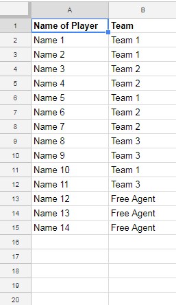
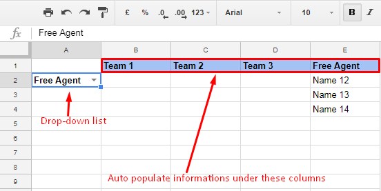
The first screenshot (Figure 1) shows the sample data, and the second screenshot (Figure 2) shows the output.
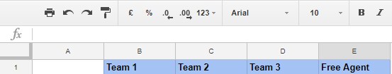
Sample Data:
Output:
You can use similar data to populate information according to your choice.
I chose this sample because I created it earlier to answer a reader’s query.
From the drop-down list, you can choose any team, such as “Team 1,” “Team 2,” “Team 3,” or “Free Agent.”
When you select a team from the drop-down, the corresponding player names will appear in the corresponding column.
I have selected “Free Agent” in the drop-down list, so the names of the corresponding players are populated below the “Free Agent” column.
If you understand the above concept, you can continue to our tutorial on how to auto-populate information based on drop-down selection.
Before starting, I want to clarify a few more things.
Skip this tutorial if you want to display a single value corresponding to your selection. For that, you can use the VLOOKUP, HLOOKUP, or XLOOKUP functions.
When you want to make a calculation based on a drop-down selection, the best way is to use the SUMIF function in Google Sheets.
Now back to the tutorial.
Steps to Auto-Populate Information Based on Drop-down Selection
Open a new Google Sheets file.
We need three tabs in this new file. Name the tabs as follows: Master Sheet, Team Members, and Team Name.
In the Team Members sheet, type the information shown in Figure 1 above (You can also use my sample Sheet shared at the end of this post.)
You can input real names under the title “Name of Player.” Mine is just a sample.
After completing the data entry, name the ranges so that you can make the formulas easy to read.
I already explained how to name ranges in Google Sheets. Please see that for details.
Here, I’m just walking you through how to name ranges for our example purpose. See the steps below:
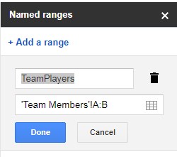
- Go to Data > Named Ranges and set the rules as shown below:
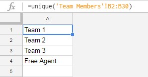
Now, go to the tab named Team Name and apply the following formula to the very first cell:
=UNIQUE('TEAM MEMBERS'!B2:B30)The result will look like the following. We can use this for drop-down selection.
Now it’s time to auto-populate information based on drop-down selection.
- To do so, go to the sheet named Master Sheet.
- Type the column headings in cells B1, C1, D1, and E1. Please refer to the above image for that.
- Now, in cell A2, we want the drop-down list. To do that, go to Data > Data validation and set the data validation rules as shown below:
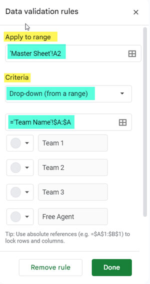
Your drop-down list is now ready.
Now, let’s move to the final steps.
When you select any team from this drop-down list, you need to populate the data range in the corresponding column. Here, data range means the name of the players.
Insert the following query formulas in cells B2, C2, D2, and E2:
Query Formulas to Automatically Populate Data Based on Drop-down Menu Item
First Formula:
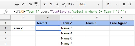
=IF(A2="TEAM 1",QUERY(TEAMPLAYERS,"SELECT A WHERE B='TEAM 1'"),"")Second Formula:
=IF(A2="TEAM 2",QUERY(TEAMPLAYERS,"SELECT A WHERE B='TEAM 2'"),"")Third Formula:
=IF(A2="TEAM 3",QUERY(TEAMPLAYERS,"SELECT A WHERE B='TEAM 3'"),"")Fourth Formula:
=IF(A2="FREE AGENT",QUERY(TEAMPLAYERS,"SELECT A WHERE B='FREE AGENT'"),"")These formulas will populate the corresponding columns with the names of the players for the selected team.
If you have done all the steps correctly, you will get the desired result.
If things are not working correctly for you, please feel free to ask me in the comments.
In this way, you can auto-populate information based on a drop-down selection in Google Sheets.
Hi Prashanth,
I’m trying to use your methods to create a sheet that cross-references the value of the drop-down menu to determine which data to display.
I want it to check the “records” sheet for a value equal to that of the drop-down value and populate several records at a time.
You can find a link to my spreadsheet, and hopefully, you’ll understand what I’m trying to achieve. I might not explain myself well in words!
You can use the following formula:
=IFNA(QUERY(QUOTES!A:H, "SELECT * where A='"&B4&"' ", 1))This formula is designed to query data from the QUOTES sheet based on the value in cell B4. If there’s anything else you need assistance with, feel free to ask.
Hi Prashanth,
I am attempting to create a spreadsheet with a drop-down menu for products. My goal is to have the Price column automatically populate when an item is selected. Despite trying various formulas for days, I haven’t had any success. Please provide assistance!
Please share the URL of a sample sheet below. I’ll do my best to help you solve the issue.
Hi Prashanth,
I hope you are still answering questions. I am trying to create a spreadsheet that, when you enter a unit number, it will auto-populate the resident’s name, income, and demographics (13 columns of information).
What I would like is for when we select the unit number for a resident, for example, #101 in column B, it will automatically populate cells C2 through M2, and so on, with their already collected information so that we don’t have to enter it every time for the same person.
Can you help?
Hi Louisa Osborn,
You might want to consider using XLOOKUP. I can assist you if you share a sample sheet.
Hey Prashanth!
Sorry, I couldn’t reply to my other comment as it’s still pending approval.
I’ve managed to sort out what I was trying to do. All I needed to do was use the basic filter function!! I was overcomplicating it all!
Hi,
That’s great to hear. I was actually waiting for your approval for edit access to your sample Sheet, but it seems that you haven’t checked your email yet.
Hi,
Thank you very much for putting this together. It’s really useful!
I’m trying to recreate it, but make things a bit more conditional and linked, if that makes sense.
I’ve amended your formula to what I want, but I know it can’t work. I’m unsure how to get it to work.
Essentially, I’m trying to create something that would be able to do the following:
=if(A2=B1:E1,query(TeamPlayers,"select A2:A15 where B2:B15='A2'"),"")Which is sort of exactly the same as you have set it up, but using the data in the cells to output the information rather than typing Team 3, etc.
Hi Matt Bee,
I believe I understand your question correctly.
Delete everything under B2:E and insert the following formula in cell B2:
=MAP(B1:E1,LAMBDA(col, FILTER('Team Members'!A2:A,'Team Members'!B2:B=col)))The formula will return a list of all the team members in the Team Members sheet who are members of the team specified in cells B1:E1.
The formula does not require a drop-down list.
Note: I have added a new hidden sheet to the shared file. You can unhide it using the “All sheets” button (three horizontal bars on the bottom left).
I hope this helps.
Hi,
I’m not sure if you’re still responding, but thank you for the templates.
I have a question. I’m creating a meal plan to track protein, carbs, fats, and calories for a day and a week. I plan to use your template and change some of the information.
I’m using the following logic statement:
=if(A2="Team 1",query(TeamPlayers,"select A where B='Team 1'"),"")The information is input vertically, but I’d like it to be displayed horizontally when an item is selected. I’d like to have a drop-down menu that pulls the protein, fats, carbs, and calories into the same horizontal line as the drop-down menu.
What would I need to change?
Hi Brandon,
You need to wrap the results with TRANSPOSE or TOROW to output the results in a horizontal row.
For example, the following formula will output the names of the players on Team 1 in a horizontal row:
=TOROW(if(A2="Team 1",query(TeamPlayers,"select A where B='Team 1'"),""))If you share your spreadsheet with sample data filled in, I would be able to give you a correct solution.
Hi,
I’m trying to create a Google Sheet where I can list all of my tasks on one tab, choose a category for the task from a dropdown, and have that task name go to the corresponding tab. I thought I had it figured out with XLOOKUP, but it is repeating each task name several times. Any suggestions?
Hi Lisa,
Thanks for your example sheet.
You need to use the FILTER function, not XLOOKUP. I’ve added the following formula in Home!G6:
=FILTER('Brain Dump'!A9:B,'Brain Dump'!C9:C="Home")Hey Prashanth!
I tried the Name Range, exactly like you did, but it doesn’t give me the result:
[URL removed by admin]
Also, do I basically need to make an IF formula statement for each country in my example? “Australia”, “Sweden”, etc.?
Thanks!
Hi Anna,
I’ve corrected the formula. If you encounter any issues, try wrapping the formula with ARRAYFORMULA.
Thanks,
Hi,
I would like to share my sheets with you. I have one master sheet and one target sheet. The master sheet contains customer names, discounts, and remarks. The target sheet has a drop-down list for the name, but when I select a name, it does not show any discounts or remarks.
Would you be able to help me troubleshoot this issue?
Hi, Reshu Sharma,
Post the URL of a copy of your sheet below in the comment.
Hi, I have to select a name from a drop-down list.
It should show the value associated with that name. If I select “Padma,” it should show his age and email address. Any help on this? How to do that.
Hi, Dev,
Use the XLOOKUP function to retrieve your required information based on the selected drop-down item.
However, XLOOKUP will only return a value from a single column. I want to retrieve both the email ID and age at the same time, which are in two different columns. If you can guide me on how to do this, I would be very grateful.
Please share a sample sheet.
Hi Prashanth,
I’m trying to make a Sheet where a movement is selected; the EF value auto-populates the score 1-4.
If nothing is selected, I need the value to equal 0. Any help would be appreciated.
Hi, Carissa,
Thanks for your Sheet and edit permissions.
You require to add IFNA to return 0 when VLOOKUP returns N/A.
Syntax:
ifna(vlookup_formula,0)I’ve added that and further modified your formula to an array formula that spills down.
Hi my friend
Is this formula wrong?
=ifs(A2="Mar 1",query(Birds,"select A where B='Mar 1'"),A2="Mar 2",query(Birds,"select A where B='Mar 2'"),"nil")
I aim to create a birding catalog. And I will constantly add conditions and values for each birding trip I complete.
In this formula, nothing shows up.
What should I do?
Hi, Ed,
Thanks for your Sheet with editable rights.
I’ve added the below solution in cell E2.
=query('birds data sheet'!A:B,"Select A where B='"&A2&"'")Hi Prashanth,
Is it possible to have a cell auto-populate data with vlookup (or another formula) dependent on what is selected from 3 different dropdown lists? I’m building a recommendations table and I want the user to be able to select A in one dropdown, B in another, and C in the third and then the column next pulls out the related info in the associated table in the same sheet.
Hi, Dani Brisebois,
Thanks for your sample Sheet.
I’ve entered my formula into your Sheet. I’ve used the FILTER() function.
Amazing! Thank you so much!! I really appreciate it!
Hi, my specific question is about pulling a name from a dropdown in column G to paste a number to column H.
Such as, if the dropdown name in cell G=Secho, then it would produce the number 93351 to appear in the H cell next to it.
I tried several tutorials, and I either cannot get it to paste, or it creates an error. Thank you very much for having this forum.
Hi, Chrys,
It depends on where you have kept the H values corresponding to G.
Here is the simplest form (H1 formula).
=SWITCH(G1,"Apple",93351,"Orange",93352,"Mango",93353,"")If the above doesn’t help, share the URL of your sample Sheet via the comments below.
That worked, thank you SO much!
Hi Prashanth,
I am trying to create a meal plan template where I select a dish (from a drop-down menu), and then it populates the list of ingredients I would need to make the said dish. I am having trouble translating your example into my page. Anyway you could help? Here is a link to view a sample of the template.
— URL Removed —
Hi, Brea,
This may work for you.
=filter({'Ingredient List'!D2:D,'Ingredient List'!C2:C},'Ingredient List'!A2:A=B5)Hello,
Is there a way I can show the list only in 1 column?
Hi, Riri,
The formula is already in “Master Sheet!G1,” and here you go!
=query(TeamPlayers,"select A where B='"&A2&"'",0)Hello,
I have a google sheet with two tabs (Master Sheet and Collateral Sheet).
I have dropdown lists for the first three columns (A, B, C) on the Collateral sheet.
The dropdown list options come from the three columns (A, B, C) on the Master Sheet.
Is there a way to pull a row of information (A-J and then U-AG) from the Master Sheet to the Collateral Sheet if you select from the dropdown list options?
Ex:
Say the Master Sheet On Row 1 states;
Column A | Column B | Column C
Chance | Property | Collateral
If I go to the Collateral Sheet Tab and select “Chance” under Column A, “Property under Column B, and “Collateral” under column C, what code would allow the Collateral sheet to pull the rest of the columns on for that row in the Master Sheet?
Does that make sense?
Hi, Chance,
I assume the drop-downs are in A1, B1, and C1 in the “Collateral Sheet.”
If so, try this formula.
=filter({'Master Sheet'!A1:J,'Master Sheet'!U1:AG},'Master Sheet'!A1:A=A1,'Master Sheet'!B1:B=B1,'Master Sheet'!C1:C=C1)YOU ARE AMAZING!!!!!!!! Thank you so much Prashanth! This formula is exactly what I was looking for 😀
Hello, I’m trying to use the drop-down function where I can select different options in multiple cells (Fan Settings), and it calculates an air quality metric that uses the sum of values associated with the combinations of what was selected.
Do you think you could help me with this? Thanks!
Hi, Kris,
I’ll try. Please share an example sheet (URL) below.
Wow! I figured it out!
Now I have a “NA” value if nothing is selected, but I need to figure out how to make it have a value of “0” rather than NA (so that I can do calculations on the table)
Hi, Richard,
Wrap the Vlookup as below.
=ifna(Vlookup_formula,0)Also, please check my array formula example in your Sheet shared with me.
Thank you very much for your help! I am going to need to study the Array formula on your page.
Is this the superior method rather than having multiple rows with repeated VLOOKUP formulas?
It certainly is cleaner for the lack of a better way of putting it.
I suppose my question would be how would you create the sheet, and the answer most likely using an array formula.
Thank you again! I am excited to learn more!
Hi,
Thank you for this useful article.
I tried your formula but got an error. Can you please look into it?
Here is the URL: — removed by admin —
Hi, Gajanan,
The issue was due to merged cells. I’ve updated the formula in your Sheet.
Oh! That’s Great! Thanks for your kind assistance.
Instead of team1, team 2, etc., I have a list of names that are in a drop-down.
I want to display the email address associated with whichever name is selected from the drop-down. So, the formula would be something like:
=IF(A2="DROPDOWN_NAME_FROM_ROW",QUERY(NAMES_LIST_TAB,"SELECT A WHERE B='DATA_FROM_EMAIL_CELL_IN_ROW'"),"")
Would this work? How can I get the IF function to work from a variable based on the Name drop-down?
Hi, Sara,
It seems you require to use a Vlookup as below.
=vlookup(A2,{names_list!B1:B,names_list!A1:A},2,0)Where;
A2 – the drop-down value.
names_list – tab name containing the list of names and email IDs.
B1:B – the column contains the list of names.
A1:A – the column contains email IDs.
Awesome! Thank you so much! Exactly what I was looking for!
Hi Prashanth,
I am creating a daily schedule that changes each day.
I want to be able to select under “Weekday” the day of the week I need to see, and then once the day is selected, the columns “Time,” “Subject,” and “Notes” populate the schedule to correspond with the day selected.
Is this possible? Here is the link to my document:
— Sheets’ URL removed —
Thank you for any help you may offer!
Dori
Hi, Dori,
Added the tab “test_II” in your sample Sheet. Please see the FILTER formula I’ve inserted there.
Hi Prasanth,
Thank you so much for this cool tutorial! I tried following your instructions, but my data isn’t populating, which I think is because I am using a horizontal format.
Could you take a look and let me know if it’s still possible to use this method?
—link/URL removed —
Thanks!
Hi, Sara,
Thanks for giving edit access. Please check the added two solutions.
Thank you so much! They work great.
Hi Prasanth,
Could you please assist me with this function?
I want a column (Probability see below) to automatically populate a percentage (predetermined) based on a selection made in a drop-down list in another column (Stage, see below).
For each of the Stage options, I have a preset % I want to be used, and that is the amount I want to auto-populate.
Percentages against each of the stages are:
Probability
0%
0%
10%
30%
Stage
1. Identify opportunity (using the list above, this would be 0%)
2. Clone opportunity (using the list above, this would be 0%)
3. Present (using the list above, this would be 10%)
4. Send RFP (using the list above, this would be 30% and so on)
Hi, Peta,
That seems possible.
Steps:
1. Enter the “Stage” values in B2:B and the corresponding “Probability” percentage values in C2:C.
2. Create the drop-down in cell E2 that contains all the “stage” values.
3. Insert the following formula in F2.
=to_percent(ifna(Vlookup(D2,B2:C,2,0)))Hi Prashanth!
It has been a game-changer! I was able to follow your tutorial to consolidate the columns into one.
I’m trying to label product status for each of my products across all stages of development (column C).
Each stage has different deliverables that I want to populate in a single column (column E).
— Sheet’s URL removed by Admin —
Hi, Jamie,
You require to use a Vlookup array formula.
=ArrayFormula({"Deliverable";ifna(vlookup(C5:C,{Deliverables!B2:B,Deliverables!A2:A},2,0))})I’ve added the above formula in cell F4.
This is amazing! Thank you so much!
Hi Prashanth
I want to create a drop-down selection box at the top of the sheet. Once the user selected the Category item from the drop-down, only the rows with the corresponding category item will be shown
—Link (Sample Sheet) removed by the admin—
How can it be done?
Thanks in advance!
Hi, Margaret,
You can either use the SLICER or the below Filter formula.
=filter(Sheet1!A4:G,Sheet1!E4:E=B1)Your column E contains the category. So created a drop-down in cell B1 to select categories from this column.
The Filter formula in cell A4 filters column E, i.e. the category, based on the drop-down selection.
The above solution provided in a copied sheet “kvp ii” in your spreadsheet. For the SLICER, please see “Sheet1”.
Thanks for your help!
I created a drop-down on “sheet 1” with list values Driver, monitor, part-time staff.
No problem with that using Data Validation.
On “sheet 2” I have values for this list of values, for example, If they select Driver from the drop-down, Driver needs to be replaced with the code 830 which will be on “sheet 2”.
That code needs to populate in the same cell.
Hope you will respond.
Hi, Ananda,
That requires Google Apps Script. Please see if this StackOverflow thread helps?
External Link.
If not, please post your question in that forum.
Best of luck.
Hi.
My dropdown list is in cell A2 and I would like the information to auto-populate in Column B2, C2, D2, and so on.
Hi, Aia,
Can you please elaborate or share a demo sheet?
Then I would be able to help you.
Hey, this is marvelous!
Is there a way to have multiple options within the same 2 cells? For example: If A1 says “Bedroom”, B1 will say “200”, but if A1 says Bonus, B1 will say 500, etc.
Hi, Tasha,
Seems you are you looking for Dependent Drop Down in Google Sheets.
I want essentially create a button to navigate the sheet. The user would select a value from the dropdown, this would trigger a function that finds the corresponding data in an adjacent column on the Master Navigation tab and populate that value with the hyperlink.
The client could then click the link to jump down to the section of the sheet they want to see. I got everything to work with this method except the hyperlink won’t carry over. Any tips?
Hi, Tartan,
I have already two tutorials on it. Please go through them.
1. Create Hyperlink to Vlookup Output Cell in Google Sheets.
2. Hyperlink to Index-Match Output in Google Sheets.
Also, please do search “Hyperlink” using the search feature on this blog for more awesome hyperlink tutorials.
Required Row 10 Vlookup with values and droplist intact. No Formula, so that I can edit & updates to master range A13:N18 dynamic row.
Hi, Jason,
Your question is not clear to me. So, please explain.
Good Day Prashanth,
Hope You can assist in this request.
1: Master sheet Vlookup at A7.
2: Row 9 normal Vlookup with formula. DONE!
3: Row 10 Vlookup result, REQUIRE to shows only values and with dropdown available. Need your help? Any method is fine as long Row 10 values and droplist available is the same copy as Row 9.
4: Row 13 – Section A to D columns “To show Only section columns” base upon any “C13:C18” drop list value selected and hide all other sections.
5: A1:G5 is your formula.
Question?
6: Required ROW 9 Vlookup with values and droplist intact. No Formula so that I can edit & updates to master range A13:N18 dynamic row.
7: M19 – Are some of the possible solutions I can think of. I prefer Method 1 solution if possible.
8: If you can email me, I can send you a video explanation in case my explanation is not clear.
Hope you can edit the formula in the Master sheets.
… link removed by admin …
Thank you so much in advance!!
Hi, Jason,
I have replaced the VLOOKUPs in cell A9:N9 with the following array formula in cell A9.
=ArrayFormula(vlookup(A7,A13:N18,sequence(1,14),0))And in cell B10 I have used a simple formula
=B9and which copied to its right.Note: I don’t know the purpose of copying the Vlookup result from row#9 to row#10. If you manually select any value in the drop-down in row#10, the formula in that cell won’t work anymore. Your requirement may meet by Google Apps Script. You can search “https://stackoverflow.com/” or ask in that community for assistance.
Hi Prashanth,
I was wondering if you were able to assist me. I am trying to find the correct formula to use to auto-populate a cell that based on 2 drop-down menu selections.
I.e. selecting a product name from drop-down menu #1, selecting the store it was purchased from in drop-down menu #2 to then give the cost price for what was selected in column 3.
I understand I need to have the data in a different tab but I’m not sure which formula to use from there… Vlookup, If??
Thank you in advance.
Hi, Lisa Juniper,
I think I can definitely help you!
There are two-three solutions (Query, Filter, or Vlookup). The better one would be a Vlookup.
Share your sheet via comment (either in View or Edit, the comment won’t be published). Please remove personal info., if any, before sharing.
I need to do this same thing with an employee roster based on the department.
So department would be team # and employees would be player plus I would need to pull in additional 5 columns of data (employee name, department, phone number, email, qualifications).
I can’t get the formula to adjust to pull in the additional columns based on A2 being the department.
Hi, Jay,
We can simply use a Filter or Query formula.
Assume the said table is in the “employee data” sheet (tab name) and the column order is employee name, department, phone number, email, and qualifications in A1:E. Obviously the first row will contain the labels.
In a blank sheet in that file create the drop-down in cell A2 and in cell B2, either you may use the Query;
=query('Team Members'!A1:E,"select * where B='"&A2&"'",1)or Filter;
={'Team Members'!A1:E1;filter('Team Members'!A2:E,'Team Members'!B2:B=A2)}to auto-populate the data based on the criterion in cell A2.
Please note the regional (File > Spreadsheet settings > Locale) settings may affect the formula (comma to semicolon issue). Read more about that here – How to Change a Non-Regional Google Sheets Formula.
Hi,
Can I combine the formulas so dependant on the drop down the text will populate in one column of cells instead of using 4 different columns?
Thanks.
Hi, Natasha Laidlaw,
Did you copy my sample Sheet? If so, in cell G1 in the ‘Master Sheet’ sheet you can see the formula for the same.
Here is that formula for your quick use.
={A2;query(TeamPlayers,"select A where B='"&A2&"'",0)}Hi Prashanth,
I have a question. I need to create 2 dropdowns depending on each other, how do I do that?
Hi, Ana,
See the Table of Content item 1.2.4.
https://infoinspired.com/google-docs/spreadsheet/data-validation-examples-in-google-sheets/
Best,
Thanks for this and this is really helpful.
What I’m trying to do is when the drop-down says “Team 1”, it displays in Column B, and when “Team 2” is selected it will replace what’s there and then show “Team 2”, and so on and so forth.
So instead of having a column for every team, I want them all in the same column but as to replace each other based on the Dropdown list. Hope this makes sense!
Hi, Mitch,
Here is the formula.
={A2;query(TeamPlayers,"select A where B='"&A2&"'",0)}I have added this in cell G1 (tab name is ‘Master Sheet’)
Alright, I was fiddling a bit with what you gave me, and I got it all working. Thanks a lot 🙂
Right, that might work, but my actual sheet got unexpected_char error. Seems I can not use this if my cells contain symbols? And If I want to expand it to 4 columns per selection?
Hi,
You are not allowed to use a mixed type of data in Query like text, numbers, date, symbols, etc in a single column.
To expand to four columns, change the +1 in the last part of the formula to +3.
If you can share a demo Sheet, I can possibly find the cause of the error.
Hi.
I want to make a dropdown menu to show different ranges of information. Like this:
So, when I change the dropdown, I get the info in the 2 columns under there.
Hi,
As per your example, the data range is D3:Q and the range D1:Q1 contains the labels for the drop-down.
So you can use the below Query in cell A3.
=Query({D3:Q},"Select Col"&match(A1,D1:P1)&",Col"&match(A1,D1:P1)+1)This formula will return two full columns based on the drop-down menu selection.
Best,
Hi Prashanth,
I am trying to make a spreadsheet where I have one tab with my ‘master data’ and one tab where, if I select an option from a drop-down menu, it populates categories with information from the master data. I have attached it here:
“Link Removed by the Admin”
I am able to make the drop-down menu, but I don’t know how to populate the value categories with information from the ‘master data’ tab.
I know there are several ways to retrieve this data but none of them seem to be working. I also want the retrieval to work even as I add new information to the master data tab.
Hi, Bella,
For that, you can use a Vlookup formula.
=ArrayFormula(transpose(vlookup(A3,'Master Database'!A1:M,{1,2,3},0)))This formula will return values from your master database column 1, 2 and 3 based on the drop-down selection.
Change this column numbers to retrieve information from other columns.
I have made a copy of your sheet. Find the formulas there.
Demo Sheet Link
Best,
Hi Prashanth,
I’m trying to do something similar, but not quite the same as what you’ve done, and unfortunately, I’m just not experienced in this.
I’d like to make a selection in a dropdown menu on one sheet, and I want to have the entire row move automatically to another tab in the sheet based on my selection.
For instance, if my dropdown selections are Blue, Yellow, Green – when I select Blue from the dropdown menu in one cell, I want that entire row to move to the tab labeled Blue. Is there a way to do this? Are you able to walk me through it?
Hi, Les,
I think we can do this. Here is one example (If I understand your question correctly)
I have the drop-down menus in Cell A1, A2, A3 … In that, I have selected “Blue” in cell A1 and A3.
We can use this Filter formula in the “Blue” tab.
=filter(Sheet1!A1:Z,Sheet1!A1:A="Blue")See if that helps. If not you can make an example sheet and drop the link in your reply below.
Best,
Hi,
Can you help me with a copy with the dropdown menus?
When I use the link, I only get the Sheet without any drop down.
Hi, Kenneth Rix,
It’s because the file is in View mode. Make a copy from the file menu to see the drop-down lists.
Hi, Kenneth Rix,
I have updated this post with the correct link and now it is set to copy mode. Sorry for the inconvenience.
That was brilliant. I was wondering if we could reverse the function where I populate a list of words that act as keywords, and when the keywords are typed in column B, column A will automatically be set to a Category which contain the keywords in column B.
It may be possible. But I can’t comment on that without seeing the data.
Is it possible to create 2 drop down lists to Auto Populate? And do I still make it unique?
Hi Luke,
I’m sorry that I couldn’t interpret your question correctly. But I’ve updated the post with the link to my sheet. You can try your luck with that sheet.
Hi Luke,
On second thought I understood your question. Following the above steps in my tutorial, it’s not possible. But as a recommended method, on a second sheet, you can easily remove the duplicates. As you may know, you can use the UNIQUE function to remove duplicates. You can have further control over the duplicate removal if you use SORTN. If you are new to Google Sheets, you can check my functions guide on the top navigation bar.
I can’t get this to work, it throws up errors on Master Sheet in Cell B2. A Parse error. I have cut and pasted it from the website but it is not working. Any ideas as to why? I would be very grateful!
Hi,
Please re-type the double quotes and try.
Thanks.
Hi,
The sheet link added at the end of the tutorial.
Cheers!
The query formulas are case-specific.
If you copy his query formulas on his working example and paste it into your example, it will work.
It took me a couple of days to figure it out, so don’t feel bad.
Hi, Troy,
That would cause a #N/A error instead of a parse error.