


")


It’s quite simple to create an Age Analysis Using Query function in Google Sheets. As I told you many times, in order to enjoy the full benefit of Google Sheets, you should learn the QUERY function. Here is my humble effort to explain to you, how to use Google Sheets Query to create an age analysis report.
Similar Tutorials:
1. Age Analysis with Pivot Table.
2. Age Analysis Using Multiple IF Logical Functions.
So let’s begin our step by step guide to create an Age Analysis Using Google Sheets QUERY Function.
Auto Generate Age Analysis Using QUERY Function in Google Sheets
Sample Data:

From the above sample data, we can prepare an age analysis using the QUERY function. If you are not following the above format in your office, please try to modify your data to match with my sample data above. But for the time being, you can create the above sample data in a new sheet to learn this trick.
In an age analysis report, the invoice values would be under categories such as Current, 30 days, 60 days, 90 days or longer period based on their aging. So that we can easily check the due payments as per our agreed payment terms with the customer or client.
Sample: Age Analysis Using QUERY Function
See a Sample Ageing Analysis Report using Query function first. Please note that I didn’t apply much formatting to the report. I only concentrate on the data and formula part.

Steps Involved in Creating an Age Analysis Report Using The QUERY Function in Google Sheets:
To use Query function to generate an age analysis report, we should first add two more columns to our sample data above. What are those two columns?
See Column E and F in the below screenshot. Therein Cell E2 and F2 you should enter different formulas as below and then copy and paste it to downwards.
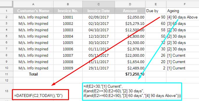
Here are that formulas:
Cell E2: I’ve entered the below DATEDIFF formula.
=DATEDIF(C2,TODAY(),"D")
Cell F2: Here I’ve entered the following formula that using Google Sheets IF Logical Function.
=if(E2<30,"[1] Current",

if(and(E2>=30,E2<60),"[2] 30 days",

if(and(E2>=60,E2<90),"[3] 60 days","[4] 90 days Above")))
Now we are set to use our QUERY formula on next sheet or same sheet to create an age analysis report. Here is that formula.
Age Analysis Using QUERY Function [Formula]
={query('Pivot Table'!A1:F10,"Select B,C, sum(D) group by B,C pivot F",1);"Total > >","",transpose(query('Pivot Table'!A1:F10,"Select sum(D) group by F label Sum(D)''",1))}
You just need to use this formula on any other tab on your’s sheet. It will instantly generate the age wise report.
Explanation to the Above Google Sheets Age Analysis Formula
I’ve used the Pivot Query Clause in the above formula to generate an age-wise analysis report.
There are two parts in the formula which you can see joined by Curly Brackets. While the first Query formula generates the Ageing Analysis Report, the second formula is intended to generate a total row at the bottom of the Query report.
If you want to dig deep into the use of Query function, I recommend you to check the below two Google Sheets guides.
1. Learn Query Function with Examples.
2. Use QUERY Function Similar to Pivot Table.
I am sharing my example sheet of Age Analysis where I’ve applied the above formulas. You can make a copy of that file from the File menu and use it as a template for your use. Any doubt, please feel free to use the comment box below. Enjoy.
Age Analysis Using Query – Access Sheet