


")


The IFS function in Google Sheets simplifies evaluating multiple conditions. It returns the answer associated with the first true condition, eliminating the need for nested IF statements.
Logical functions are fundamental tools for spreadsheet users. Beginners often start with aggregation functions like SUM and AVERAGE, but quickly progress to mastering essential logical functions such as IF, IFS, AND, NOT, and OR.
These functions enable diverse tasks like checking conditions, making decisions, and handling errors. The IFS function excels in these areas.
Unlike its counterpart, the IF function, which needs nesting (putting one IF inside another) for many conditions, IFS can handle lots of conditions at once. This makes it simpler and more organized to deal with multiple conditions without complicating your formulas.
IFS Logical Function: Syntax and Arguments
Syntax:
IFS(condition1, value1, [condition2, value2, …])In this syntax, condition1 and value1 are required arguments; others are optional.
Arguments:
condition1: A condition that evaluates to TRUE or FALSE.value1: The returned value ifcondition1is TRUE.condition2,value2, …: Additional conditions and values if the preceding ones are evaluated to be false.
What happens when condition1 evaluates to FALSE and condition2 is not specified?
The formula will return #N/A.
Unlocking the Power of IFS: Examples in Google Sheets (with Images)
Here are a couple of examples to help you get familiar with using the IFS logical function in Google Sheets.
Basic Examples
Let’s consider a scenario where cell A1 contains the name of a student, and cell B1 contains his total marks out of 1000.
You want to get the result “Selected” in cell C1 if his marks are greater than or equal to 500.
Here is how you use the IFS function:
=IFS(B1>=500, "Selected")If his marks are less than 500, the formula may return #N/A, indicating no match. To remove the #N/A error, you can specify condition2 that evaluates to TRUE, like 1=1, and specify value2 or leave value2 blank:
=IFS(B1>=500, "Selected", 1=1,)The formula above will return “Selected” if the value in cell B1 is >=500; otherwise, it returns blank instead of #N/A. To return “Rejected” instead of blank, specify value2 as below:
=IFS(B1>=500, "Selected", 1=1, "Rejected")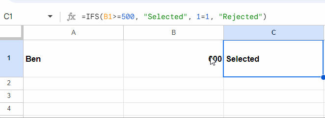
Related: How to Specify a Value When the Logical Expression is FALSE in IFS.
Points to be noted:
- If
value1,value2,… are text or special characters, enclose them within double quotes. - If
value1,value2,… are numbers, do not use double quotes. - If
value1,value2,… represent date, time, or timestamp, specify them using relevant date functions or a combination of functions:- Date:
DATE(year, month, day) - Time:
TIME(hour, minute, second) - Timestamp:
DATE(year, month, day) + TIME(hour, minute, second)
- Date:
Using DateTime as Output (value1):
Here’s an example using the IFS function with DateTime as the output (value1):
=IF(B1<600, DATE(2023, 12, 12)+TIME(10, 30, 0))This will return “12/12/2023 10:30:00” if the value in B1 is less than 600. To return any text with the date, you can use the JOIN function:
=IF(B1<600, JOIN(,"Appointment Date is ", DATE(2023, 12, 12)+TIME(10, 30, 0)))It will return “Appointment Date is 12/12/2023 10:30:00”.
You can also use Date, Time, or DateTime in the condition part of the IFS function:
=IFS(A1>DATE(2030, 12, 25), "Upcoming Event")Or use functions like TODAY(), NOW() in both condition and value parts:
=IFS(A1>TODAY(), "Future Date", 1=1, TODAY())I hope these basic examples help you understand the use of the IFS logical function in Google Sheets.
Multiple Conditions in IFS Function
An effective way to learn about the use of multiple conditions in an IFS function is through a classic past, present, and future example. This example not only helps in understanding multiple conditions but also introduces a nested IFS formula.
Formula:
=IFS(B2<TODAY(), "Past", B2=TODAY(), "Present", B2>TODAY(), "Future")Explanation:
B2<TODAY(): This condition checks if the date in cell B2 is earlier than today. If true, the formula returns “Past.”B2=TODAY(): This condition checks if the date in cell B2 is the same as today’s date. If true, the formula returns “Present.”B2>TODAY(): This condition checks if the date in cell B2 is later than today. If true, the formula returns “Future.”
An advantage of this logical test when learning the IFS function is that it avoids returning #N/A unless cell B2 contains an error. It opens up possibilities for exploring the IFS function. Even if cell B2 is blank or contains any value other than a date, the formula will still return one of “Past,” “Present,” or “Future.”
To address scenarios where cell B2 is blank or contains a value other than a date, we can use a nested IFS formula. This will be discussed in the next section below.
Nested IFS in Google Sheets
To assess whether the value in a cell is a date in Google Sheets, one effective method is using the DATEVALUE function.
As a side note, for Excel users, this approach is specific to Google Sheets and doesn’t apply to Excel.
Here’s how it works:
The expression DATEVALUE(B2) returns a serial number representing the date in cell B2 or an error. Wrapping it with IFERROR will return either a blank or a number.
So, you can use IFERROR(DATEVALUE(B2)) as condition1 (the first condition) in IFS and another IFS formula as value1.
=IFS(
   IFERROR(DATEVALUE(B2)),
      IFS(B2<TODAY(), "Past", B2=TODAY(), "Present", B2>TODAY(), "Future"),
   1=1,
      "Value is not a valid date"
)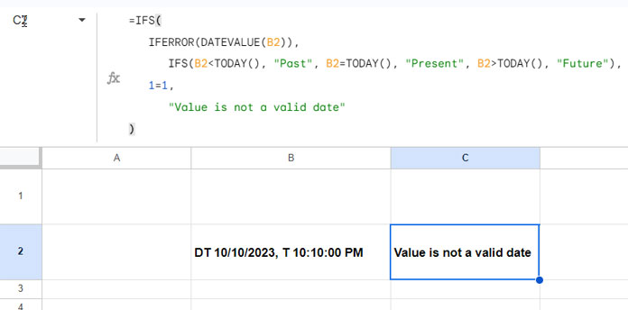
Breaking down the nested IFS formula:
condition1:IFERROR(DATEVALUE(B2))value1:IFS(B2<TODAY(), "Past", B2=TODAY(), "Present", B2>TODAY(), "Future")condition2:1=1value2:"Value is not a valid date"
Using Complex Logic in the IFS Function in Google Sheets
The IFS function allows for complex logic using functions such as AND, OR, and NOT. Here are some examples:
Assuming there are scores in A1:C1, the following IFS formula, in combination with the AND function, tests if all the conditions are TRUE:
=IFS(AND(A1>60, B1> 60, C1> 60), "Good")This formula evaluates a set of conditions and returns “Good” only if all three conditions (A1>60, B1>60, C1>60) are TRUE.
Similarly, the following IFS formula, in combination with the OR function, tests if at least one of the conditions is TRUE:
=IFS(OR(A1>60, B1> 60, C1> 60), "Good")This formula returns “Good” if any of the conditions (A1>60, B1>60, C1>60) is TRUE.
The next IFS formula combines AND and OR logical functions:
=IFS(OR(AND(A1>60, B1>60), AND(A1>60, C1>60), AND(B1>60, C1>60)), "Good")In this formula, it uses the OR function to evaluate if any of the conditions AND(A1>60, B1>60), AND(A1>60, C1>60), AND(B1>60, C1>60) is TRUE. In short, if any of the two scores are greater than 60, it returns “Good.”
Similar: Combined Use of IF, AND, and OR Logical Functions in Google Sheets.
In all these formulas, the false result will be #N/A. You can handle this by adding a default condition using IFS or wrapping the entire formula with an IFERROR function.
Examples:
=IFS(AND(A1>60, B1>60, C1>60), "Good", 1=1, "Poor")
=IFERROR(IF(AND(A1>60, B1>60, C1>60), "Good"), "Poor")
Related: How to Properly Utilize AND and OR Functions with IFS in Google Sheets.
Substituting IFS with Nested IF Statements in Google Sheets
We can replace the IFS function with nested IF functions in Google Sheets. Also, it has an edge over IFS in some cases.
In certain situations, the IFS function cannot return an array result, requiring the use of IF or VLOOKUP, as explained in my tutorial: How to Use IFS Function to Return an Array Result in Google Sheets.
Here, we are going to learn how to use nested IF instead of an IFS formula.
In the following example, we have a drop-down in cell B1 containing the items “Tea,” “Coffee,” and “Milk Shake.”
IFS Formula:
=IFS(B1="Tea", 1.5, B1="Coffee", 2, B1="Milk Shake", 5 )Nested IF Formula:
=IF(B1="Tea", 1.5, IF(B1="Coffee", 2, IF(B1="Milk Shake", 5 )))The above formulas will return 1.5, 2, and 5 if the selected value in cell B1 is “Tea,” “Coffee,” or “Milk Shake,” respectively.
Conclusion
In this tutorial, I have covered everything that one requires to master the IFS logical function in Google Sheets.
You can use either IF or IFS for logical tests in Google Sheets. Of the two, IFS is more reader-friendly because the alternative nested IF can be difficult to read, depending on the number of conditions.
In addition to these two, you can also consider the SWITCH function if the condition doesn’t involve comparison operators.
Hope you are doing well.
This ASIN has 4 item codes cause to sell this ASIN we need 4 different items. How can I get the 4 items to pull through and put on Sheet 5 that I send out without doing it manually?
I need the formula to fetch the details from one sheet to another sheet. I herewith attached a google sheet link for your kind reference.
—link removed by admin—
Please help with it for me.
Thanks.
Saravanan.
Hi, Saravanan,
I can’t do much in a VIEW-only sheet. You may please try your luck with this formula.
=Query({{Sheet4!A2:A,Sheet4!B2:D};{Sheet4!A2:A,Sheet4!E2:G};{Sheet4!A2:A,Sheet4!H2:J};{Sheet4!A2:A,Sheet4!K2:M}},"Select * where Col2 is not null order by Col1",0)I haven’t seen the quantity column either.
Thanks, Prashanth, Thanks for the formula. It works fine.
Hi, Prasanth,
Thanks for giving the solution to the earlier problem. I have another 2 problems need to solve.
Problem 1:
Column L – I need “Yes” to appear when Column H is greater than or equal to $1000 and Column G is greater than or equal to 12%. When in between $0-$1000 and over 12% say “Potential”
Problem 2:
The next formula is pulling across only ASINS that say “Yes” in column L (“prashanth info inspired”), over to column A in “Sheet3”.
I herewith attached the same Google Sheets which is you did already.
Hi, Saravanan,
This time the Sheets’ setting is in “View”. So I couldn’t insert my formulas.
The formula for Problem 1:
Please make L2:L6 blank. Then paste this formula in cell L2 only.
=ArrayFormula(if((H2:H6>=1000)*(G2:G6>=12%)=1,"Yes",if(isbetween(H2:H6,0,1000)*(G2:G6>12%)=1,"Potential","No")))In this, you can see the use of a new Google Sheets function called ISBETWEEN.
Problem 2:
Use this FILTER formula in Sheet3.
=filter('prashanth info inspired'!D2:D6,'prashanth info inspired'!L2:L6="Yes")Thanks so much, Prashanth. It works well.
Hi, Prasanth,
What I am after is column G must be less than 577 to continue to check for light and small.
If the package weight (H) is less than 113, then the light and small fee will be $1.97.
If it is greater than 113, but less than 284, then the light and small fee will be $2.39. Otherwise, it will be $0.00.
If this fix, it will be helpful for me.
Thanks.
Saravanan
Hi, Saravanan,
See the below formula in cell I2 (which copied down).
=if(and(lt(G2,577),lt(H2,113)),1.97,if(and(lt(G2,577),gte(H2,113),lt(H2,284)),2.39,0))
The tab name in your file is “prashanth info inspired”.
Wanted to correct my question: The nested IF contains only 3 conditions…if I use more than 3, it throws out an error ‘expecting 2 or 3 arguments but got 5 or 6….or 13 whatever that is.’
Apologies for double posting
Hi, Arvind,
In the IF function, there are only 3 arguments. They are;
1. logical_expression
2. value_if_true
3. value_if_false (optional)
IF arguments explained:
=ArrayFormula(if(A1="veg",VEGGIES,if(A1="fru",FRUITS,)))Here
A1="veg"is the logical_expression.VEGGIESis the value_if_true.If the value in A1 is not matching “veg”, then the formula will execute the value_if_false part, which is another IF formula. That means we can nest IF formulas using the value_if_false argument.
You are getting the error as you are nesting wrongly. Here is one more example to correct nesting.
=if(A1=1,"one",if(A1=2,"two",if(A1=3,"three",if(A1=4,"four",if(A1=5,"five","?")))))
Do include the ArrayFormula when using named ranges.
Best,
Hi Prashanth,
Thanks for the clarification; actually my query is a bit related to the number of nested IF that the IF statement can allow.
I read somewhere and also observed that the maximum number of IF statements one can nest is 7, and in the project, I am working I have about 14 conditions.
I tried using the IFS formula, but it does not return the named range. For eg, if A1=”veg”, then it returns ONLY the 1st element of the range VEGGIES, whereas with the IF statement I get the whole 4X5 matrix (in both cases, I used the ArrayFormula).
Is there some limitations to the output of IFS?
Regards
Hi,
I was trying to point out the error in your formula.
I don’t know the maximum number of nested IF allowed in Google Sheets. I tested up to 40 nested IF and I found it working flawlessly. I know Google Sheets IF can accept more than 40 nested IF statements. I left there due to time constraints.
Here is one example: You can test this by changing the value in cell A1 1-40.
=if(A1=1,1,IF(A1=2,2,IF(A1=3,3,IF(A1=4,4,IF(A1=5,5,IF(A1=6,6,IF(A1=7,7,IF(A1=8,8,IF(A1=9,9,IF(A1=10,10,
IF(A1=11,11,IF(A1=12,12,IF(A1=13,13,IF(A1=14,14,IF(A1=15,15,
IF(A1=16,16,IF(A1=17,17,IF(A1=18,18,IF(A1=19,19,IF(A1=20,20,
IF(A1=21,21,IF(A1=22,22,IF(A1=23,23,IF(A1=24,24,IF(A1=25,25,
IF(A1=26,26,IF(A1=27,27,IF(A1=28,28,IF(A1=29,29,IF(A1=30,30,
IF(A1=31,31,IF(A1=32,32,IF(A1=33,33,IF(A1=34,34,IF(A1=35,35,
IF(A1=36,36,IF(A1=37,37,IF(A1=38,38,IF(A1=39,39,IF(A1=40,40,
IF(A1=41,41)))))))))))))))))))))))))))))))))))))))))
Regarding IFS, it won’t populate an array result.
Hey Prashanth,
Thank you very much! I guess I must have made a nesting error. I tried to find a work-around for this by breaking down the formula into three parts of 4 IF statements each in different cells and then write an IF statement referring to these cells. I guess it works well now.
Thank you for your patience! 🙂
Best
Arvind
Welcome 🙂
Hi Prashanth,
Thank you for the clarifications. I have a slightly different question: I want to display a named range based on the text in, say, cell $A$1, and I want to do this based more than 10 conditions in Google sheets. Now I used IFS along with the Arrayformula but it only displays the first cell when the condition occurs whereas when I use nested IF statements then it displays the entire named range.
Eg: I have one named range with vegetables and relative size, weight and price (called VEGGIES) and another with fruits (FRU) and I want to check the cell $A$1 to see if it contains the partial match ‘veg’ then return the entire named range.
Can you help me here?
Hi Prashanth,
Great article, but I’m still having some trouble with what I’m trying to do. My goal is to calculate a total price based on whether the product is Expensive/Cheap (F5) and the number of orders (0-4) (E5). I’m looking to get the following results:
If someone buys the Expensive product, their total price is $100 multiplied by their number of orders.
If someone buys the Cheap product and has 0-3 orders, their total price is $20 multiplied by their number of orders.
If someone buys the Cheap product and has 4 orders, their price is $60 total, the same price as if they had 3 orders.
I’ve tried a number of different functions, including IF, IFS, both nested and otherwise and it’s just not coming together. My last attempt looked something like this:
=IFS(F5="Expensive",100*E5,AND(F5="Cheap",E5<"4"),20*E5,AND(F5="Cheap",E5="4"),60)
Unfortunately, when I set E5 to 4 and F5 to Cheap, it still gives me $80 instead of $60 like it's supposed to. What am I doing wrong?
Hi, Alex,
Try this formula.
=if(F5="Expensive",E5*100,if(and(F5="Cheap",E5<4),E5*20,if(and(F5="Cheap",E5=4),60,)))
Hi,
Thanks for your feedback !!
I want the final status to be either “Complete” or “In-progress”, right now the ArrayFormula is outputting several statuses across the column. Any way to overcome this?
Regards,
Hi, Nirmala,
I think this simple formula will work.
=ArrayFormula(if(or(A6:K6="Complete",isblank(A6:K6)),"Complete","In progress"))If not, please feel free to share an example sheet.
Hi, can I use IFS with Characters? (trying to say if any of the values between A6 and K6 are either “Complete” or BLANK, the status is “Complete” otherwise its “In Progress”).
eg :
IFERROR(IFS({A6:K6}="Complete","Complete",{A6:K6}="","Complete"),"In Progress")Hi, Nirmala,
IF works well with ArrayFormula. So you can use that function as below.
=ArrayFormula(if((A6:K6="Complete")+(isblank(A6:K6))=1,"Complete","In Progress"))Best,
Hi, I’m trying to get nested ifs to function with a custom function that was an addon.
The spreadsheet is for a game I play.
The formula I tried was
=IF(A2="","",=IF(D2=0,(=EVEPRAISAL_ITEM(B2)),D2/C2))So basically I want it to check A2 and if empty leave empty box, however, if A2 has a date in it, it checks if d2 has the number 0 in it (as that column is total cost spent on items). If it’s 0 then get minimum sell from EVEPRAISAL_ITEM, however, if it has a price other than 0 then divide that with the quantity bought to get the price per item.
Hi, David,
Please try this formula.
=if(len(A2),if(D2=0,EVEPRAISAL_ITEM!B2,D2/C2),)Best,