This post explains how to remove duplicate records using the UNIQUE function and its purpose in Google Sheets.

You can utilize the Data > Data cleanup > Remove duplicates feature to permanently eliminate duplicate values from a selected range. However, there are instances where you might want to retain the original list and create a new list without duplicates.

The UNIQUE function facilitates the filtering of unique values into a new range, providing a basic solution for removing duplicate content in rows or columns.

For more advanced operations, you may explore alternatives such as SORTN or the previously mentioned Remove duplicates Data menu option.

The primary goal of removing duplicate values using the UNIQUE function is often to obtain unique values for operations like SUMIF, SUMIFS, COUNTIF, COUNTIFS, etc.

Common Causes of Duplicate Records in Spreadsheets

Duplicate records in spreadsheets can arise from various factors, depending on the nature of your work and your experience in using spreadsheets. Here are some of the most common reasons for duplicates:

1. Copy-Pasting Data: Copying and pasting data is a common practice in spreadsheets. Care should be taken to avoid inadvertently introducing duplicate entries or risking data loss.
2. Data Entry Errors: Manual data entry is prone to mistakes. Oversights during input can lead to accidental duplicate records.
3. Collaborative Editing: In collaborative environments where multiple users access the same sheet, the possibility of duplicate entries increases.
4. Sheet connected to Google Forms: Multiple submissions through Google Forms can result in duplicates if not managed appropriately.
5. Unstacking of Data: When unstacking data using formulas, duplicate values in one or more columns are common as part of data integrity and manipulation.

Implementing best practices, careful data handling, and utilizing spreadsheet functionalities wisely can help minimize and address issues related to duplicate records.

It’s important to note that removing duplicates using the UNIQUE function compares rows or columns in a multi-column range, not individual cells.

Removing Duplicate Rows Using the UNIQUE Function in Google Sheets

Explore a list of some of my favorite books and authors.

The sample data is in B3:D8, where column B contains the names of the authors, column C contains their book titles, and column D contains the year of publication. I intentionally included Agatha Christie’s “A Pocket Full of Rye” twice.

Let’s see how to remove this duplicate content using the UNIQUE function in Google Sheets.

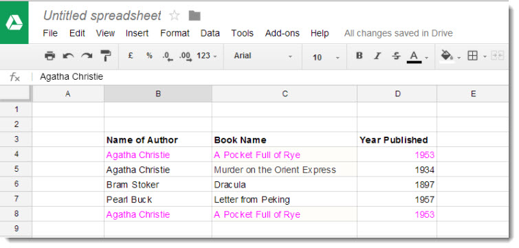
Note: The above screenshot was captured from Google Sheets years ago. That’s why you see a different logo in the top left corner. I’ve kept this screenshot unchanged for nostalgic reasons.

Insert the below formula in cell E3 to remove the last row in the range, which is a duplicate:

=UNIQUE(B3:D8)

The above formula considers values in the entire row for duplicates.

For example, if the ‘Year Published’ differs in both highlighted rows, the output will contain all records. In such cases, there won’t be anything to remove from the range.

Removing Duplicate Columns Using the UNIQUE Function in Google Sheets

Most of us keep the data orientation as shown above. Some built-in features like grouping, filtering, etc., work with data arranged in rows. The SUBTOTAL function will only exclude hidden rows in aggregation, not hidden columns. So, row-wise data is always preferred.

However, in rare cases, we may arrange data in columns.

What about removing duplicates in columns using the UNIQUE function in Sheets?

The data in the following example is the same as the one above, but the orientation is different. I mean, the records are now arranged in columns instead of rows.

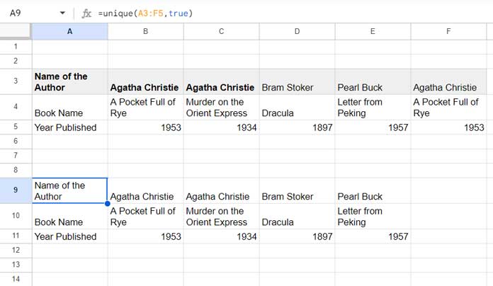
We can use the following UNIQUE formula in cell A9 to remove duplicates in the range A3:F5:

=UNIQUE(A3:F5, TRUE)

Where:

• range: A3:F5
• by_column: TRUE

As per the syntax UNIQUE(range, [by_column], [exactly_once]).

Removing Duplicates and Real-life Applications

Other than data clean-up, the primary role of using the UNIQUE function is to remove duplicate records attributed to conditional count, sum, average, etc.

In the following example, we have appliance names, brands, models, and prices in the range A2:D6.

The UNIQUE formula in cell F2 below removes duplicate appliance names in the cell range A2:A6:

=UNIQUE(A2:A6)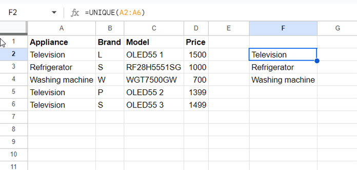

To get the total price of each appliance, we can use the following SUMIF formula in cell G2:

=ArrayFormula(SUMIF(A2:A6, F2:F4, D2:D6))

In cell H2, enter the following COUNTIFS formula to get the count of products:

=ArrayFormula(COUNTIFS(A2:A6, F2:F4))

Enter the following AVERAGEIF formula in cell I2 and drag it down to get the average price of each product:

=AVERAGEIF($A$2:$A$6, F2, $D$2:$D$6)

So, in real life, you can leverage the UNIQUE function to eliminate duplicates and apply the obtained result in other functions for conditional aggregation.

Conclusion

In simpler terms, the UNIQUE function serves two main purposes:

1. Tidying up data sets by eliminating duplicate items in rows or columns.
2. It is particularly useful when dealing with unique records in more complex operations that involve counting, summing values, calculating averages, and similar tasks.

One thing is evident from the examples above: incorporating the UNIQUE function into your data manipulation tactics opens up new possibilities for efficiency and accuracy.

Experiment with its diverse applications to enhance your data analysis capabilities.