


")


We can use the Format > Custom number format to add custom text to numbers in Google Sheets with calculation support.
Adding text to a number is quite easy with a simple function called CONCATENATE or using the ampersand (&) symbol. There are also more advanced text join functions in Google Sheets like JOIN and TEXTJOIN.
However, these functions (approaches) have two drawbacks:
- If you add text to a number using a function or the ampersand symbol, the returned value will be text, even if the original value was a number. This means that you cannot use the result in calculations.
- Adding text to a number using a function or the ampersand symbol requires an additional cell to use the formula.
For example, if you have the value 12500 in cell A1 and you want to add the text “(approx)”, you can use the following formula in cell B1:
=A1&" (approx)" // returns 12500 (approx)To add text to a number and retain the number formatting, you need to use the Custom number format feature in the Format menu.
How to Add Custom Text to Numbers in Google Sheets (Calculation Support)
Steps to add custom text to numbers that can be considered in the calculation:
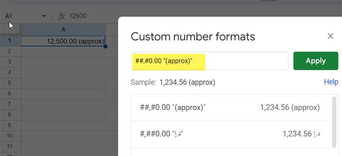
- Select the cell(s) that you want to format. For example, let’s select cell A1.
- To open the Custom number formats dialog box, click Format > Number > Custom number format.
- In the Custom number format field, enter
##,#0.00 "text". Replacetextwith the text you want to suffix to the number. Let’s use(approx). So the code will be##,#0.00 "(approx)". - Click Apply.
How to check if the returned value is a number:
- Select the cell and see the value in the formula bar. It will be just the number without text.
- Alternatively, you can use the following ISNUMBER formula in any other cell:
=ISNUMBER(cell_reference)This will return TRUE if the value in the specified cell is a number, else FALSE.
For example, if you enter the following formula in cell B1:
=ISNUMBER(A1)And cell A1 is formatted with the custom number format ##,#.00 "(approx)", then the formula in cell B1 will return TRUE, because the value in cell A1 is a number, even though it is also formatted with text.
Anatomy of the Google Sheets Custom Number Format Code
Google has a detailed article on custom number, date, and time formats. You can check it out here when you have time: Date & number formats.
That being said, let’s understand the code that we have used to add custom text to numbers and retain the formatting:
##,#0.00 "text"Tokens:
"text"token: Displays whatever text is inside the quotation marks as a literal. In our example, the text is"(approx)".#token: Represents a digit in the number. An insignificant 0 digit is not rendered. So if a cell contains just 0, it won’t return that.0token: Represents a digit in the number. An insignificant 0 digit is rendered. If a cell contains just 0, it will return that..(period) token: Represents the decimal point in the number.,(comma) token: Groups by the thousands.
You can use this code by replacing “text” with the custom text or symbol that you want to add to the number.
It’s useful when you want to add text like “approx” or “lump sum” to numbers and use them in calculations. If we didn’t have this feature, we would have to type/insert the text in an adjoining cell corresponding to the number.
Conclusion
Adding custom text to numbers has another use in Google Sheets: you can use it to create custom currency formats. This is useful if you need to use a currency that is not supported by Google Sheets by default.
Related: How to Set Your Country’s Currency Format in Google Sheets.
For example, if you want to use the currency symbol د.إ (UAE Dirham [AED]), you can use the following code:
#,##0.00 "د.إ"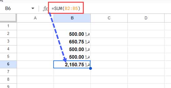
This code will format the number in the cell with two decimal places and add the text "د.إ" to the end of the number. However, Google Sheets already includes most currencies.
You can use custom currency formats in any cell in Google Sheets, and they will be included in calculations.