You can save time entering data into spreadsheets by intelligently using certain commands and formulas. Combining text and date, while retaining the date format, is one common use case. In this Google Docs Spreadsheet tutorial, you can learn how to simplify data entry. You will learn the following tips:
- How to combine text in one cell with text in another cell.
- How to combine text in one cell with a number in another cell.
- How to combine text in one cell with the date in another cell.
I have included two additional tips, points #1 and 2.
Like in Microsoft Excel, you can use the CONCATENATE function to combine text in one cell with text/number/date in another cell in Google Docs Spreadsheets.
Why are all these required?
First, let us take a look at the benefit of this function. In the following similar scenarios, we can use the CONCATENATE function or equivalents:
Join the item code with numbers and letters: In this case, you can simplify data entry by entering the numbers in one column and the text in another column, and then combining them. This way, you can quickly complete the data entry and avoid reducing your typing speed by entering text and numbers (alphanumeric values) in the same column.
Add prefix/suffix text to dates: You can follow the same logic as above. Enter all the dates in one column and the text you want to prefix/suffix to the date in another column. This way, you can complete your tasks on or before the scheduled time.
Now to the tips:

How to Combine Text in One Cell with Number in Another Cell
There are different functions and formulas that can be used to combine values in different cells. I am using the ampersand (&) symbol in this example, but here are a few other supported functions: Difference Between JOIN, TEXTJOIN, and CONCATENATE Functions in Google Sheets.
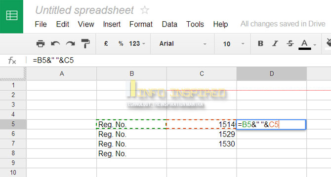
The screenshot below shows how to use the ampersand symbol to join the contents of two cells:
=B5&" "&C5
This formula will put a space between the contents of the two cells. If you do not want to add a space, you can omit the quotation marks. The formula will then look like this:
=B5&C5In this example, you would enter the formula in cell D5 and then copy it down to the other cells in the column. However, it is more efficient to use an array formula, which will expand the result itself. The following array formula can be used to combine the values in cells B5:B and C5:C:
=ArrayFormula(B5:B&C5:C)Simply enter this formula in cell D5 and you do not need to copy it down to the other cells in the column.
I have not included an additional space in this array formula, but you can add one by using an additional ampersand.
How to Combine Text in One Cell with Text in Another Cell
Follow the same steps as above. The formula is also the same.
However, this is rarely required, and there is no specific benefit to doing so. I usually use it to combine first and last names.
How to Combine Text in One Cell with Date in Another Cell
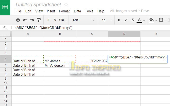
In this example, we are combining text, text, and date using the ampersand (&) symbol, just like above. However, we need to use the TEXT function for the date. Do you know why?
When you combine a date with text or two dates, the date will lose its formatting. To retain the date format, use the TEXT function.
See the screenshot for details.

You can copy the formula downwards to apply it to multiple cells. But if you are looking for an array formula, here it is:
=ArrayFormula(IF(LEN(A5:A),(A5:A&" "& B5:B&"-"&TEXT(C5:C,"DD/MM/YY")),))Two Common Issues When Combining Text and Date in Google Sheets (and How to Fix Them)
You may face two issues when combining text and date using the ampersand (&) in Google Sheets, especially when using a delimiter (separator).
- If the date cell is blank, the formula will return the date “30/12/1899”. This is a common issue with blank cells, which we have discussed earlier in this tutorial: How to Return Blank Instead of 30-12-1899 in Google Sheets Formulas.
- The delimiter will be added irrespective of the presence of values.
Solutions
Solution to issue 1:
If cell A2 contains the name “Ben” and cell B2 contains the date “17/10/2000” (his date of birth), the following formula will return the string “Ben’s date of birth is on 17/10/2000”:
=A2&"'s date of birth is on "&IFERROR(TEXT(DATEVALUE(B2),"DD/MM/YYY"))If B2 is empty, it will not return “Ben’s date of birth is on 30/12/1899”. Instead, it will return “Ben’s date of birth is on”.
How does the formula work?
The DATEVALUE function returns an error when B2 is blank or any value other than a date. Eventually, the TEXT function will return the same error. The IFERROR function removes this error.
This way, we can solve the blank date cell issue when we combine text and date in a Google Docs spreadsheet.
Solution to issue 2:
If you want the formula to only return a value if both cells have values, then use the following formula:
=IF(LEN(A2)*LEN(B2),A2&"'s date of birth is on "&TEXT(B2,"DD/MM/YYY"),)This way, we can avoid the delimiter text appearing when there is no value to combine.


Can someone help me? Nothing works.
“Starting Date: (44766) / Ending Date: (44768) / Workers: (4) / Hours: (8) / Days to Complete: (32) / Days: (1) / Days Remaining: (-9)”
Start Date | End Date | workers | hours | Days “C” | Days | Days “R”
AY4 | AZ4 | BA4 | BB4 | BC4 | BD4 |BE4
7/24/2022 | 7/26/2022 | 4 | 8 | 32 | 1| -9
Hi, Rich,
This formula may work.
="Starting Date: ("&text(AY4,"MM/DD/YYY")&") / Ending Date: ("&text(AZ4,"MM/DD/YYY")&") / Workers: ("&BA4&") / Hours: ("&BB4&") / Days to Complete: ("&BC4&") / Days: ("&BD4&") / Days Remaining: ("&BE4&")"Need help too. I want to show 08:00-16:00
But the raw data is 0900-1300. How can I turn it to 08:00-16:00 using a formula?
Hi, Sandi,
If the value 0900-1300 is in cell B2, the following formula can format it to 09:00-13:00.
=REGEXREPLACE(REGEXREPLACE(B2,"^.{2}", "$0:"),"^.{8}", "$0:")I don’t know the logic to convert it to 08:00-16:00. Is there any specific pattern?
Needing Help!!! I am attempting to create a spreadsheet for student grades and I need to have the dates above.
I want it to show (1/3/2021 – 1/9/2021) in each column and progressively continue in the respective row with the dates. How can I do this? I’ve gotta be doing something wrong…HELP!
Hi, Mr. Hayes,
Can you please share a sheet that contains just sample data the demonstrates the problem?
You can use the ‘reply’ to share the link.